Bucharest University of Economic Studies IDA Institute Digital Assets Blockchain Research Center AI4EFin Artificial Intelligence for Energy Finance Romanian Academy, Institute for Economic Forecasting MSCA Digital Finance
“The building blocks of the Sharpe ratio—expected returns and volatilities—are unknown quantities that must be estimated statistically and are, therefore, subject to estimation error. This raises the natural question: How accurately are Sharpe ratios measured?” — Lo (2002)
Sharpe ratios, Jan 2015 – Sep 2026: Bitcoin 1.05, S&P 500 (Standard & Poor's) with dividends 0.82, gold 0.76
standard error (SE) of each: about 0.29
S&P 500 minus gold Sharpe ratio: \(+0.06\)
95% interval \([-0.65,\ +0.88]\): the data do not rank the two assets
SE of the S&P 500 annualised mean return over 11.7 years: 5.1 percentage points (pp)
None of the 10 pairs of non-crypto assets stays significant after a Bonferroni correction
The building blocks of the Sharpe ratio—expected returns and volatilities—are unknown quantities that must be estimated statistically and are, therefore, subject to estimation error. This raises the natural question: How accurately are Sharpe ratios measured?
The chapter asks two questions: which financial comparisons can we trust, and how precisely do we know them. Lo (2002) poses the second question for the Sharpe ratio: the means and volatilities of returns are not observed but estimated, so any ranking built from them also carries their estimation errors. The chapter covers market structure, the history of exchanges and of financial models, the course data and the basic measurements: returns, the compound annual growth rate (CAGR), annualised volatility and drawdown, each with its precision.
Over the common window 2 January 2015 – 18 September 2026, the S&P 500 (Standard & Poor's) with dividends has a CAGR of 13.7% and an annualised volatility of 17.6%, gold 11.8% and 16.3%, and Bitcoin 60.6% and 66.7%. The Sharpe ratios are 1.05 for Bitcoin, 0.82 for the S&P 500 and 0.76 for gold, each with a standard error (SE) of about 0.29. The standard error of the S&P 500 annualised mean return, estimated from 11.7 years of data, is 5.1 percentage points.
The difference between the Sharpe ratios of the S&P 500 and gold, computed by a bootstrap on common days, is +0.06, with 95% interval [−0.65, +0.88]. The data are compatible both with an advantage of 0.65 for gold and with one of 0.88 for the S&P 500, so the comparison is inconclusive. None of the 10 pairs of non-crypto assets stays significant after a Bonferroni correction. The risk–return chart describes the sample; it does not rank expected returns.
Return and risk of the main asset classes, 2 January 2015 – 18 September 2026: on the vertical axis the CAGR, the realised compound growth, on the horizontal axis the annualised volatility, on a log scale; everything in USD (US dollar) except EUR (euro)/RON. Interactive chart: “Risk and Return, 2015–2026 (1/2)” →
What you will be able to do
Compute returns, CAGR, annualised volatility and maximum drawdown.
Interpret a price series before using it: the price field, the observation time and bad ticks.
Compute the change in the correlation of two assets between two periods, on common days.
Compute a mean return and a Sharpe ratio with a standard error and a 95% interval.
Interpret an empirical claim and spot a misleading one, including an AI-generated (Artificial Intelligence) one.
Data ConventionsThe course data sources, survivorship bias and the choice of price and calendar.
Measurement and PrecisionReturns, CAGR, annualised volatility, volatility drag, drawdown and the precision of the expected return and of the Sharpe ratio.
The 2000–2026 LandscapeRisk and return across asset classes, the significance of the ranking, crises and drawdowns, the VIX (CBOE Volatility IndeX) and time-varying correlations.
The Romanian MarketThe Bucharest Stock Exchange and the BET (Bucharest Exchange Trading, index) index, 1997–2026.
The opening section states the two questions of the chapter and of the course, describes how the course is organised and assessed, and introduces the AI-assisted research loop that every chapter closes with. The empirical material starts in the next section.
Almost every statement in empirical finance is a comparison: one asset grew faster than another, one strategy had a higher Sharpe ratio, a correlation rose after a given date. The chapter asks two questions about such statements:
Which comparisons can be trusted at all, given how prices are recorded, which data are kept and which are lost.
How precisely the quantities being compared are known, since every mean, volatility or Sharpe ratio is an estimate computed from a finite sample.
The chapter has two parts. Part I describes the structure of markets, the history of exchanges and of financial models, the course data and the basic measurements, each with its precision. Part II looks at the evidence for 2000–2026, at the Romanian market, at digital assets and passive investing, and at two case studies. The chapter closes with one complete pass of the research loop assisted by artificial intelligence (AI).
Detailed examples and advanced topics are collected in Further Topics, after the Conclusions.
In brief
Markets, Data and Models
Guiding questions
which financial comparisons can we trust?
how precisely do we know them?
Part I: market structure and the history of exchanges and models
the course data, measurement and its precision
Part II: the 2000–2026 evidence and the Romanian market
digital assets, passive investing and two case studies
Closing: one full pass of the research loop assisted by artificial intelligence (AI)
Detailed examples and advanced topics are in Further Topics, after the Conclusions
the footer button leads there, and the Back button returns to the slide you came from
The chapter is paired with Seminar 0, and its exercises define what the reader should be able to do afterwards. The first two groups of exercises are:
Computational: simple and log returns, the compound annual growth rate (CAGR), annualised volatility and maximum drawdown.
About the data themselves: before a price series is used, one must know which price field it contains, at what time each price was observed and whether it contains bad ticks, and every cleaning decision must be justified.
The remaining exercises concern inference. The change in the correlation of two assets between two periods is computed on the days common to both series. A mean return and a Sharpe ratio are reported with a standard error and a 95% confidence interval, not as bare point estimates. The last exercise asks the reader to judge an empirical claim, including one produced by an AI assistant, and to identify what makes it misleading: missing uncertainty, an ignored rival explanation, a wrong formula or a wrong reference.
The Further Topics and the Appendix are reading for familiarity.
In brief
What you should be able to do (Seminar 0 exercises)
compute returns, CAGR, annualised volatility and maximum drawdown (A1–A4, B2)
The course belongs to the master's programme Applied Statistics and Data Science, 2026/2027, of the Faculty of Cybernetics, Statistics and Economic Informatics at the Bucharest University of Economic Studies (ASE). The lectures are given by Prof. Daniel Traian Pele and the seminars by Antoaneta Amza, PhD (Doctor of Philosophy) candidate.
The final grade has three components. The team project, consisting of a GitHub repository, a presentation and an oral defence, carries 70%. Quizzes and seminar activity carry 20%; there is one quiz per chapter on the course website, with 20 questions drawn from a bank and an explanation for each answer. Attendance carries 10% and requires at least 4 lectures and 4 seminars, recorded with the code of the day shown in the room as a QR (quick-response) code or through the Attendance form on the website.
In brief
Master's programme Applied Statistics and Data Science, 2026/2027
Faculty of Cybernetics, Statistics and Economic Informatics
The project is carried out in teams of 3–4 students, each team working on one research question with real market data; the projects are presented in Chapter 19. Each team keeps one public GitHub repository, with a README that states the question, the data and how to run the code, and with commits every week. Every figure is published as a Quantlet: one folder holding the code, a `Metainfo.txt` file and the chart.
The governing rule is reproducibility. A result counts only if someone else can reproduce it from the repository: the data are loaded by code, every reported number is produced by a script, and random computations use a fixed seed. The tools are Python, Google Colab and the course repository, with the libraries pandas, numpy, scipy, statsmodels, scikit-learn and matplotlib.
The use of AI tools is allowed, on condition that it is declared. Every use is recorded in the file `AI_USE.md`, and every error of an AI tool that the team caught is recorded in `AI_ERRORS.md`.
In brief
Teams of 3–4 students, one research question on real market data
The research loop of the course has six steps: literature, hypothesis, data and code, robustness, critique and report, after which the report feeds the next round of reading. An AI assistant, typically a large language model (LLM) such as Claude, ChatGPT or Gemini, can produce a draft at every step: a map of the literature, competing hypotheses, code, a plan of robustness checks, or a hostile referee report on the team's own work.
The division of responsibility is fixed. The researcher owns the question, the identifying assumption, the test and every reported number, and verifies each transition of the loop. The verification checklist has three items:
Every reference has a DOI (Digital Object Identifier) that resolves and a title that matches;
Every number is reproduced from the data by the team's own code;
The null hypothesis \(H_0\), the test, the sample and the correction for multiple testing are fixed before the results are seen.
The checklist answers the typical failures of LLMs in research:
They invent references that look plausible;
They write formulas that are plausible but wrong;
They produce code with look-ahead, using information from the future at the date of a forecast;
Asked repeatedly, they search until some result is "significant".
Each of these failures has a corresponding check in the list: the DOI check catches invented references, independent reproduction catches wrong formulas and look-ahead, and fixing the test in advance limits the search for significance. The final section of the chapter runs the loop on a new question.
The chapter's two questions, which comparisons can be trusted and how precisely they are known, run through all that follows. The project rules and the research loop translate them into practice: every number must be reproducible, and every claim, whether written by a person or by an AI tool, must survive the same checks.
The Financial System and Market Structure
This section describes who trades in financial markets, what is traded and how a traded price is formed. The last point matters for everything that follows: the price downloaded from a data vendor is the outcome of a particular trading mechanism at a particular time, and its noise depends on that mechanism.
A financial market is a mechanism for exchanging claims on future cash flows: shares, bonds, currencies, contracts and tokens. The diagram shows the basic flows. Savers, such as households and pension funds, pass money to intermediaries, such as asset managers, banks and brokers, who channel it as capital to issuers, firms and governments. The issuers give the savers claims in return. Intermediaries trade through venues and infrastructure: exchanges, dealers, clearing houses and custodians.
The section answers two questions: who trades what, and where; and how the price that we later download is formed.
Markets perform three economic functions: capital allocation, risk sharing, and payments and settlement. Two properties determine how well they do so. Liquidity is the ability to convert assets into cash quickly. Price discovery is the process by which prices aggregate information that is dispersed among many participants.
Participants are usually divided into two sides. The buy side consists of investors and asset managers, who can be passive, replicating an index, or active, trying to beat it. The sell side consists of brokers, who execute orders on behalf of clients, and dealers, who trade from their own inventory. A market maker is a dealer who continuously quotes a price at which it will buy and a price at which it will sell.
The table groups the traded instruments into seven classes, by their cash flows and their main risks. Equities give dividends and a residual claim on the firm, with market and firm-specific risk. Fixed income, government and corporate bonds, pays coupons and principal and carries interest-rate and credit risk. The money market holds instruments with maturities below one year, such as Treasury bills (T-bills) and repos, secured loans, whose main risk is liquidity.
The foreign-exchange (FX) market trades currencies; EUR/RON, for instance, is the number of lei per euro, and its cash flow is the interest differential between the two currencies. Commodities, such as gold and oil futures, pay no cash flow; a futures position earns or loses a roll yield, the gain or loss from replacing an expiring futures contract with the next one. Derivatives, futures, options and swaps, have contingent payoffs and carry leverage and counterparty risk. Digital assets, such as Bitcoin, Ether and stablecoins, have no cash flow or a protocol-specific one, and are exposed to high volatility and regulatory risk.
An exchange-traded fund (ETF) is a fund whose shares trade on an exchange like a stock. Despite the differences between the classes, the course applies one statistical toolbox to all of them: returns, volatility, dependence and tails. The full list of terms is in the Appendix.
In brief
Class
Examples
Cash flow
Main risks
Equities
shares, equity ETFs
dividends, residual claim
market, firm-specific
Fixed income
government and corporate bonds
coupons, principal
interest rate, credit
Money market
T-bills (\(<\) 1 year), repo (secured loan)
short-term interest
liquidity
FX
EUR/USD, EUR/RON
interest differential
currency, policy
Commodities
gold, oil futures
none (roll yield)
supply, storage
Derivatives
futures, options, swaps
contingent payoffs
leverage, counterparty
Digital assets
Bitcoin, Ether, stablecoins
none / protocol-specific
volatility, regulation
Terms in the table
ETF (exchange-traded fund): a fund whose shares trade like a stock
FX: the currency market; EUR (euro)/RON = lei per euro
roll yield: the gain or loss from replacing an expiring futures contract
One statistical toolbox for all of them: returns, volatility, dependence and tails
On most exchanges trading is organised around a limit order book: the list of all waiting buy orders (bids) and sell orders (asks), sorted by price. In the stylised book of the figure, the best bid is 99.99 and the best ask is 100.01. The bid–ask spread is the difference between the best ask and the best bid, here \(100.01 - 99.99 = 0.02\); it is the price paid for trading immediately. Depth is the quantity available near the best prices.
Orders differ in whether they supply or consume liquidity. A limit order rests in the book at a chosen price and provides liquidity to others. A market order executes at once against the orders in the book and consumes liquidity. A stop order becomes a market order when the price reaches a trigger level; when many stop orders are clustered at similar levels, their execution can accelerate a fall.
The second panel follows a market buy order of 5 units through the same book. The order first takes the 2 units offered at the best ask, 100.01, and then 3 of the units offered at the next level, 100.02 (highlighted in orange). Its average execution price is therefore \((2 \times 100.01 + 3 \times 100.02)/5 = 100.016\), above the best ask quoted before the trade.
After the trade, the best ask has moved to 100.02, and the spread has widened from 0.02 to 0.03. The change in price caused by the order itself is market impact, treated in Chapter 10. Even this small example shows that the price at which a trade is recorded depends on the size of the order and on the state of the book.
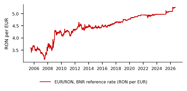
A "daily price" is a price observed at a specific time, and that time differs across markets. For exchange-traded assets it is usually the closing auction: for the S&P 500, at 20:00 or 21:00 UTC (coordinated universal time). In a call auction, orders are collected over an interval and matched at one price. Bitcoin trades continuously and has no close; the price of day \(t\) is taken at 24:00 UTC, the end of day \(t\). For EUR/RON the course uses the reference rate of the National Bank of Romania (BNR, Banca Națională a României), fixed around 13:00 Bucharest time.
The venue also determines what is recorded. Exchanges, over-the-counter (OTC) dealers, dark pools and crypto platforms that trade 24/7 show different prices and different trades for the same asset. The Appendix contrasts auctions with continuous trading, explains why speed is rewarded and tabulates the venues.
In brief
A “daily price” is a price observed at a specific time
exchange-traded assets: the closing auction (S&P 500: 20:00 or 21:00 UTC, coordinated universal time); in a call auction, orders are collected and matched at one price
auctions versus continuous trading, and why speed is rewarded: Appendix
Bitcoin: no close; the price of day \(t\) is taken at 24:00 UTC, the end of day \(t\)
EUR/RON: the reference rate of the BNR (Banca Națională a României, the National Bank of Romania), fixed around 13:00 Bucharest time
The venue decides what is recorded (venue table in the Appendix)
exchanges, OTC (over-the-counter) dealers, dark pools and 24/7 crypto platforms show different prices and trades
Different observation times split the same news across two days. If one market closes before a piece of news and another after it, the news enters the return of the first asset one day later than that of the second. Correlations computed from daily closes of such assets are therefore attenuated; the Appendix gives an example.
A second source of noise is the bid–ask bounce. Trades alternate between the bid and the ask, so observed price changes are negatively autocorrelated even when the efficient price follows a random walk. In the model of Roll (1984), with \(p_t\) the observed trade price, \(\Delta p_t = p_t - p_{t-1}\) its change and \(s\) the bid–ask spread,
By (0.1), a wider spread gives a more negative covariance of consecutive price changes; the derivation is in the Appendix.
Spreads, market impact and the fragmentation of trading across venues all add noise to observed prices. The effect is most visible at high frequency, the subject of Chapters 9 and 10.
In brief
Different observation times split the same news across two days (Appendix)
correlations of assets with different closes are attenuated
Bid–ask bounce: trades alternate between bid and ask
observed price changes are negatively autocorrelated, even when the efficient price is a random walk
the Roll model: consecutive price changes have a negative covariance, \(\operatorname{Cov}(\Delta p_t, \Delta p_{t-1}) = -s^2/4\) (Roll (1984); derivation in the Appendix)
\(p_t\): the observed trade price; \(\Delta p_t = p_t - p_{t-1}\): its change; \(s\): the bid–ask spread; a wider spread gives a more negative covariance
Spreads, impact and fragmentation add noise to observed prices
most visible at high frequency (Chapters 9 and 10)
Section summary
A downloaded price is the outcome of a trading mechanism at a given time and venue. The spread, the depth of the book and the observation time all leave traces in the data: bid–ask bounce produces negative autocorrelation, and different closing times attenuate correlations. These effects must be kept in mind whenever two series are compared.
A Short History of Markets and Financial Models
This background section follows two parallel histories: that of exchanges and the crashes that accompanied them, and that of the financial models built to understand prices and risk. Each wave of models answered a question raised by the markets of its time, and most of them reappear in later chapters of the course.
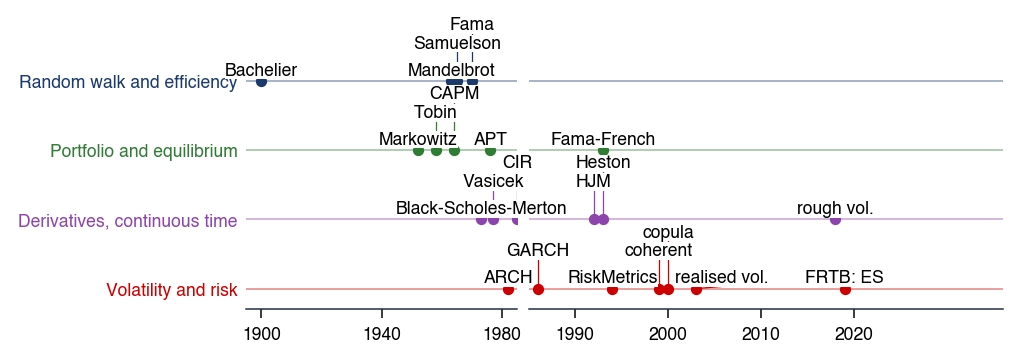
The timeline places the main events on one axis of years. The upper lane, in blue, shows the founding of exchanges and the first traded securities; the lower lane, in red, shows bubbles, panics and crashes. The section asks how exchanges, crashes and models developed together, and what each wave of models added.
The chart supports two observations. Shares have traded continuously since the 1600s, and bubbles and crashes followed almost immediately after the first continuous trading. The Bucharest Stock Exchange opened in 1882; its history is in the Appendix.
Question for the room The selected year is 1602, when trading in VOC (Vereenigde Oostindische Compagnie, Dutch East India Company) shares begins. Which episode appears first after this year on the ‘Bubbles, panics and crashes’ lane?
Answer
Tulip mania, in 1637, 35 years after 1602. The Mississippi and South Sea bubbles occur in 1720, and the panic in 1792. The Bucharest Stock Exchange opened in 1882.
In the interactive version, the slider sets the last year shown, from 1250 to 2026, and the ▶ button advances the timeline year by year. The events appear in order on their lanes, so the gap between the first exchange events and the first episodes of the lower lane can be read directly.
In brief
This background section answers
how did exchanges, crashes and models grow together?
what did each wave of models add?
The chart: the horizontal axis shows years
top (blue): exchanges and the first traded securities
bottom (red): bubbles, panics and crashes
Shares have traded continuously since the 1600s, and bubbles and crashes followed almost at once
The Bucharest Stock Exchange opened in 1882 (Appendix)
The exchange as an institution emerged in the Low Countries. In Bruges, between the 13th and the 15th centuries, merchants met on the square in front of an inn of the Van der Beurse family (Gelderblom, 2013); the name gave the words bourse, beurs and bursă. In Antwerp, in 1531, a building was erected purposely for daily trading (Gelderblom, 2013).
The decisive step came in Amsterdam. In 1602 the Dutch East India Company, the VOC (Vereenigde Oostindische Compagnie), issued transferable shares. Within a decade the market for these shares had continuous trading, forward contracts, options and short selling (Gelderblom & Jonker, 2004),(Petram, 2014). The engraving shows the Amsterdam exchange built by Hendrick de Keyser, in 1612.
In London, organised trading in securities grew between 1698 and 1773 (Neal, 1990). John Castaing published lists of prices at Jonathan's Coffee House, and in 1773 the brokers called their new building the Stock Exchange.
In New York, on 17 May 1792, 24 brokers signed the Buttonwood Agreement (Sylla, Wright & Cowen, 2009), the origin of the New York Stock Exchange (NYSE). Between Amsterdam and New York, the main elements of a modern exchange were therefore in place: a fixed venue, transferable securities, published prices and a closed group of intermediaries.
The early history of markets is also a history of bubbles. During the tulip mania in Holland, 1636–37, the prices of contracts on tulip bulbs rose many-fold and collapsed in February 1637. Later research describes a smaller episode than the legend, with few bankruptcies (Garber, 1989),(Goldgar, 2007). In 1720, the Mississippi Company in Paris, led by John Law, and the South Sea Company in London rose and collapsed within months. Frehen, Goetzmann & Rouwenhorst (2013) describe 1720 as a bubble around a real innovation, Atlantic trade and insurance.
Panics brought the first public interventions. In the panic of 1792 in New York, the Treasury under Alexander Hamilton acted as a lender of last resort (Sylla, Wright & Cowen, 2009). In 1873 crashes occurred in Vienna, in May, and in New York, in September; the NYSE closed for ten days, and the US (United States) contraction dated by the National Bureau of Economic Research (NBER) lasted until 1879.
The 20th century added Black Tuesday, the New York crash of 1929, described in the Appendix, and 19 October 1987, when the Dow Jones Industrial Average (DJIA) fell 22.6% in one day, with large falls in every major market (Roll, 1988). The episodes share recurring ingredients: a new asset or technology, credit and leverage, and then forced selling. Bubbles and crashes are the subject of Chapter 17.
In brief
Tulip mania, Holland 1636–37: prices of bulb contracts rose many-fold, then collapsed in February 1637
The first question that financial models addressed was whether past prices predict future prices. The benchmark answer is the random walk for the log price,
\[\ln P_t = \ln P_{t-1} + \mu + \varepsilon_t,\]
(0.2)
where \(\mu\) is a constant drift and the shocks \(\varepsilon_t\) are independent and identically distributed (iid) with mean zero. Bachelier (1900) modelled prices with Brownian motion. Mandelbrot (1963) showed that price changes have far heavier tails than under the Normal distribution. The efficient market hypothesis (EMH) of Fama (1970) states that prices fully reflect the available information; under (0.2), past prices carry no information about future changes beyond the drift.
The second question was which risks should earn a reward. Markowitz (1952) proposed choosing portfolio weights by the mean and variance of the portfolio return, which makes diversification depend on the covariances between assets. The capital asset pricing model (CAPM) of Sharpe (1964) concludes that in equilibrium only market risk is priced. These ideas are developed in Chapters 1–4; the Appendix gives the history in more detail.
Can past prices predict future prices? Random walk and efficiency (Appendix)
a random walk for the log price: \(\ln P_t = \ln P_{t-1} + \mu + \varepsilon_t\), with iid (independent and identically distributed) zero-mean shocks \(\varepsilon_t\)
The next wave asked what an option is worth. Black & Scholes (1973) and Merton (1973) showed that a continuously rebalanced hedge in the stock and the riskless asset replicates the option. The option price is therefore fixed by the absence of arbitrage, and it does not depend on the expected return of the stock.
A second question was whether volatility is forecastable. The ARCH model (AutoRegressive Conditional Heteroskedasticity) of Engle (1982) and its generalisation GARCH (Generalised AutoRegressive Conditional Heteroskedasticity) by Bollerslev (1986) make today's variance depend on past shocks. They explain volatility clustering: large returns tend to be followed by large returns, of either sign.
The third question came from regulation: how much capital should a bank hold against market risk (BCBS, 1996), (BCBS, 2019)? The first answer used the Value-at-Risk at level 1% (VaR 1%), the loss that is exceeded with probability 1%. The later framework uses the expected shortfall at level 2.5% (ES 2.5%), the mean loss in the worst 2.5% of cases. These models are developed in Chapters 5–12.
ARCH (AutoRegressive Conditional Heteroskedasticity) and GARCH (generalised ARCH): today's variance depends on past shocks, which explains volatility clustering
The crisis of 2008 is an example of model risk, the risk that the model used for pricing is wrong. A collateralised debt obligation (CDO) is a bond paid from a pool of loans, divided into tranches with different priority. In market practice a single parameter of a Gaussian copula priced every tranche of a CDO. That parameter could not reproduce the joint defaults observed in the crisis, so the prices of the tranches understated the risk of losses spreading across the pool.
The Appendix describes the Gaussian copula and 2008 in more detail, and also the development of interest-rate models, from Vasicek to the yield curve.
In brief
Lesson of 2008: an example of model risk (Appendix)
CDO (collateralised debt obligation): a bond paid from a pool of loans
one Gaussian-copula parameter priced every tranche of a CDO
the parameter could not reproduce the joint defaults of the crisis
Interest-rate models, from Vasicek to the yield curve: Appendix
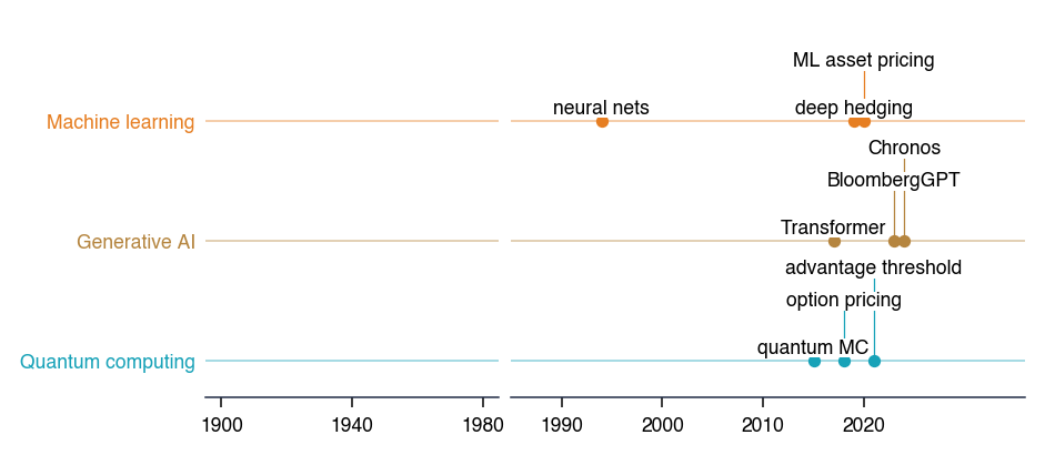
Financial Models (4/4): Learning from Big Data and Text
The most recent wave responds to a problem of scale: hundreds of firm signals and millions of documents do not fit a small parametric model. Machine learning (ML) fits flexible functions to data and selects them by out-of-sample performance rather than by theory. In Gu, Kelly & Xiu (2020), trees and neural networks beat linear models in forecasting the returns of about 30,000 US stocks using 94 firm characteristics. The monthly out-of-sample \(R^2\) stays below 1%, a small number that is nevertheless economically valuable.
Generative AI rests on the Transformer architecture of Vaswani et al. (2017), which underlies today's large language models. Lopez-Lira & Tang (2026) find that ChatGPT scores of news headlines predict next-day stock returns out of sample. Foundation models for time series forecast new series without retraining (Ansari et al., 2024).
The main risks of these methods are:
Overfitting;
Look-ahead, because a language model may have read texts written after the forecast date;
Many trials on the same data.
These methods and their risks are treated in Chapters 13–15. The appendix on quantum computing is linked from the slide.
In brief
Problem: hundreds of firm signals and millions of documents do not fit a small parametric model
Machine learning (ML; Appendix): flexible functions fitted to data
selected by out-of-sample performance rather than by theory
Gu, Kelly & Xiu (2020): trees and neural networks beat linear models on about 30,000 US stocks and 94 firm characteristics
the monthly out-of-sample \(R^2\) stays below 1%: small but economically valuable
Each wave of financial models answered a question posed by the markets: whether prices are predictable, which risks are priced, what an option is worth, how volatile tomorrow will be, how much capital a bank needs, and how to learn from large data sets and text. The crashes show that models also fail, and 2008 is the clearest example of model risk.
Data Conventions
This short section fixes the data used throughout the course and the conventions for the price field and the calendar. Two series that differ only in these conventions can lead to different conclusions, so the conventions are stated before any measurement.
Where the Course Data Come From, and Survivorship Bias
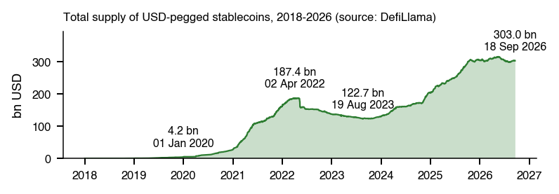
The course uses four data sources. Daily market data from EODHD (EOD Historical Data), covering indices, stocks, ETFs, FX, crypto and yields, are saved once as CSV (Comma-Separated Values) files in the course repository. FRED (Federal Reserve Economic Data) provides US interest rates, exchange rates and macroeconomic series as public CSV files. The BNR publishes the official RON (Romanian leu) reference exchange rates as public XML (eXtensible Markup Language) files. DefiLlama provides the stablecoin supply and data on decentralised finance (DeFi) as public JSON (JavaScript Object Notation).
Any data set built today carries a risk of survivorship bias (Brown, Goetzmann, Ibbotson & Ross, 1992). A sample rebuilt from the assets or funds that still exist today omits those that failed or were closed, and therefore makes past returns look too good. The bias matters most for comparisons across long periods and for universes from which weak members drop out.
In brief
Data
Content
Format
Daily market data from EODHD (EOD Historical Data), saved in the course repository
For stocks and ETFs, the course uses the adjusted close, which corrects for dividends and splits;
For indices, FX and crypto, the close;
For bonds, the closing quoted yield.
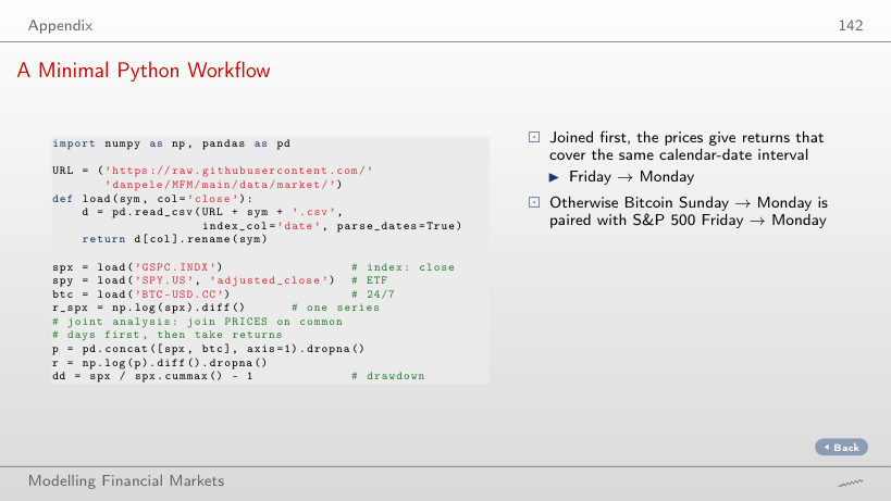
The calendar must be handled with care when several series are combined. A single series is analysed on its own calendar. For several series, the prices are first joined on the days common to all of them, and returns are computed afterwards; returns computed first on different calendars would span different intervals.
Annualisation uses the observed frequency, the number of returns per year actually present in the data. This is about 365 for crypto, which trades every day, 260 for spot gold and 252 for equities.
In brief
Price type
stocks and ETFs: the adjusted close (dividends, splits)
indices, FX and crypto: the close
bonds: the closing quoted yield
Calendar
one series: returns on its own calendar
several series: join the prices on common days first, then take returns
Annualise with the observed frequency, the number of returns per year in the data
about 365 for crypto, 260 for spot gold, 252 for equities
Measurement and Precision
This section defines the basic measurements of growth and risk, simple and log returns, the CAGR, annualised volatility and drawdown, and then asks how precisely they are known. The examples use the S&P 500 and the SPY (SPDR S&P 500 ETF Trust) ETF over 2015–2026. The main result is that the precision of a mean return or of a Sharpe ratio depends on the number of years in the sample, not on the number of observations.
The two definitions aggregate in different directions. Simple returns aggregate across assets: a portfolio with weights \(w_i\) has return \(R_{p,t} = \sum_i w_i R_{i,t}\) exactly. Log returns aggregate over time: the \(h\)-day log return is the sum \(r_{t+1} + \dots + r_{t+h}\). Portfolio calculations therefore use simple returns, and calculations over time are easier with log returns.
For small moves the two returns nearly coincide, since by (0.3)\(r_t = R_t - R_t^2/2 + \dots\). For large moves they differ considerably: a fall of 50% is a simple return of \(-50\%\) but a log return of \(\ln 0.5 = -69\%\).
In brief
This section answers
how do we measure growth and risk?
how precisely do we know the answer?
The simple return \(R_t\) and the log return \(r_t\)
A price index, such as the S&P 500 or BET, the main index of the Bucharest Stock Exchange, ignores dividends. A total-return index, such as BET-TR, and the adjusted close of a stock or ETF reinvest them. Comparisons of long-run growth must use the same kind of series on both sides.
Over \(T\) days, daily simple returns multiply and log returns add:
where \(Y\) is the sample length in years, measured as calendar days divided by 365.25, and the ratio \(P_{\text{end}}/P_{\text{start}}\) is the multiple. The second form of (0.4) states that the CAGR is the sum of log returns per year, expressed as a simple rate.
For the S&P 500 price index from 2 January 2015 to 18 September 2026, the sample spans 4,277 calendar days, so \(Y = 4\,277/365.25 = 11.71\) years. The index rose by a multiple of 3.72, which gives \(\mathrm{CAGR} = 3.72^{1/11.71} - 1 = 11.9\%\) a year.
In brief
A price index (S&P 500, BET) ignores dividends
BET: the main index of the Bucharest Stock Exchange
the total-return index (BET-TR) and the adjusted close reinvest them
The subscript \(d\) marks a daily quantity and the subscript \(A\) an annualised one; \(A\) also denotes the number of returns per year actually observed. The annualised volatility scales the daily standard deviation by \(\sqrt{A}\):
\[\hat\sigma_A = \hat\sigma_d\sqrt{A},\]
(0.5)
where \(\hat\sigma_d\) is the sample standard deviation of daily log returns.
The square root follows from the aggregation of log returns. The one-year log return is the sum of \(A\) daily log returns; if these are uncorrelated and have constant variance \(\sigma_d^2\), the variance of the sum is \(A\sigma_d^2\), and its standard deviation is \(\sigma_d\sqrt{A}\). When daily returns are autocorrelated, the scaling in (0.5) is no longer exact; the variance ratio, which measures the departure, is in the Appendix.
For SPY, the SPDR (Standard & Poor’s Depositary Receipts) S&P 500 ETF with dividends, the sample has \(T = 2\,944\) daily returns over \(Y = 11.71\) years, so \(A = T/Y = 251.4\) returns per year.
In brief
The subscript \(d\) marks a daily quantity, the subscript \(A\) an annualised one
\(A\) is also the number of returns per year actually observed
Annualised volatility: \(\hat\sigma_d\) scaled by \(\sqrt{A}\)
\[
\hat\sigma_A = \hat\sigma_d\sqrt{A}
\]
\(\hat\sigma_d\): the sample standard deviation of daily log returns
why \(\sqrt{A}\): the one-year log return is the sum of \(A\) daily returns; if these are uncorrelated with constant variance, the variance of the sum is \(A\sigma_d^2\)
with autocorrelated daily returns the scaling is no longer exact (variance ratio, Appendix)
Example: SPY has \(T = 2\,944\) daily returns over \(Y = 11.71\) years, so \(A = T/Y = 251.4\)
SPY: the SPDR (Standard & Poor’s Depositary Receipts) S&P 500 ETF, with dividends
The annualised arithmetic mean \(\hat\mu_A = A\,\bar R\), where \(\bar R\) is the sample mean of daily simple returns, is larger than compound growth. The two are linked by
The reason is the expansion \(r_t \approx R_t - R_t^2/2\): averaging over days, the mean of \(R_t^2\) is about \(\sigma_d^2\), and annualising gives (0.6). The term \(\hat\sigma_A^2/2\) is the volatility drag: at the same arithmetic mean, higher volatility lowers compound growth.
For SPY over 2015–2026, computed from simple returns, \(\hat\mu_A = 14.39\%\) and \(\hat\sigma_A = 17.53\%\), so the right-hand side of (0.6) is \(14.39\% - 17.53\%^2/2 = 12.85\%\). The CAGR of SPY is 13.7%, and \(\ln(1.137) = 12.84\%\): the approximation reproduces the observed compound growth.
The S&P 500 price index has a CAGR of 11.9% over the same period, 1.8 percentage points (pp) a year less than SPY. The gap comes mainly from reinvested dividends, net of the ETF's fees and tracking differences.
In brief
The annualised arithmetic mean \(\hat\mu_A = A\,\bar R\) exceeds compound growth
Volatility does not say how much an investor lost from the best earlier moment, because it does not depend on the order of returns, while losses from a peak do. The drawdown measures the percentage distance of the price below its running peak:
The maximum drawdown (MDD) is the deepest fall from a peak over the whole sample. The duration of a drawdown is the number of days until the price exceeds the earlier peak again.
The example of Seminar 0 uses the prices 100, 120, 90, 110, 130, 100. The running peak is 100, 120, 120, 120, 130, 130, and (0.7) gives the drawdowns 0, 0, \(-25\%\),\(-8.3\%\), 0 and \(-23.1\%\). The maximum drawdown is \(-25\%\), although the last price is above the first.
In brief
Volatility does not say how much an investor lost from the best earlier moment
the order of returns matters
Drawdown: the percentage distance below the running peak
Assume that daily simple returns \(R_t\) are iid, with true mean \(\mu_d\) and standard deviation \(\sigma_d\), and that the sample has \(T = AY\) observations. The annual mean is estimated by \(\hat\mu_A = A\,\bar R\), with \(\bar R = \frac{1}{T}\sum_{t=1}^{T} R_t\).
The standard error (SE) is the typical distance between \(\hat\mu_A\) and the true annual mean. Since \(\operatorname{Var}(\bar R) = \sigma_d^2/T\),
The second form of (0.8) is the important one: the SE falls only with the square root of the number of years. A 95% confidence interval for the annual mean is \(\hat\mu_A \pm 1.96\,\operatorname{SE}\).
In brief
Assumption: the daily simple returns \(R_t\) are iid
true mean \(\mu_d\) and standard deviation \(\sigma_d\)
\(T = AY\) observations
Estimator: \(\hat\mu_A = A\,\bar R\), with \(\bar R = \frac{1}{T}\sum_{t=1}^{T} R_t\)
Standard error (SE): the typical distance between \(\hat\mu_A\) and the true annual mean
For SPY over 2015–2026, \(\hat\mu_A = 14.4\%\),\(\sigma_A = 17.5\%\) and \(Y = 11.71\) years; the volatility is computed from simple returns, and from log returns it is 17.6%. Formula (0.8) gives \(\operatorname{SE} = 17.5\%/\sqrt{11.71} = 5.1\) pp, and the 95% confidence interval for the annual mean return is \([4.3\%,\ 24.4\%]\). Almost twelve years of daily data thus leave a wide interval for the expected return.
The question for the room asks which would halve this SE: four times as many observations, for example hourly instead of daily data, or four times as many years. By (0.8) the SE depends only on the span \(Y\), not on the sampling frequency (Merton, 1980). Halving it requires four times as many years, about 47 instead of 11.7.
The Sharpe ratio (SR) is the mean return per unit of risk; in this chapter the risk-free rate is set to 0. Per day it is \(\mathrm{SR}_d = \mu_d/\sigma_d\), the ratio of the mean to the standard deviation (SD) of daily simple returns, and annualised it is \(\mathrm{SR}_A = \sqrt{A}\,\mathrm{SR}_d\). The value estimated from the sample is \(\widehat{\mathrm{SR}}_A\).
Like the mean, the Sharpe ratio is an estimate with a standard error. For iid returns following the Normal distribution, Lo (2002) gives
With daily data the term \(\mathrm{SR}_A^2/(2A)\) is tiny, \(0.82^2/504 \approx 0.001\), so by (0.9) the SE depends almost only on the number of years \(Y\). The Further Topics discuss the precision of the Sharpe ratio when the risk-free rate is not zero.
In brief
Sharpe ratio (SR): the mean return per unit of risk, with the risk-free rate set to 0
per day \(\mathrm{SR}_d = \mu_d/\sigma_d\) (mean and standard deviation, SD, of daily simple returns); annualised \(\mathrm{SR}_A = \sqrt{A}\,\mathrm{SR}_d\)
\(\widehat{\mathrm{SR}}_A\): the value estimated from the sample
Its standard error, for iid returns following the Normal distribution (Lo (2002)):
Returns, the CAGR, annualised volatility and drawdown are simple to compute, but each depends on conventions: simple or log returns, price or total-return series, the observed number of returns per year. Their precision is limited by the span of the sample: the standard error of a mean return and of a Sharpe ratio falls only with the square root of the number of years. Over 11.7 years, the 95% interval for the annual mean return of SPY runs from 4.3% to 24.4%.
The 2000–2026 Landscape
The previous section defined the measurements and their precision. This section applies them to the main asset classes on a common window: what return and what risk each class delivered, whether any ranking between them is statistically significant, how deep the crises of 2000–2026 were, how volatility moves between regimes and how the correlations that drive diversification change over time.
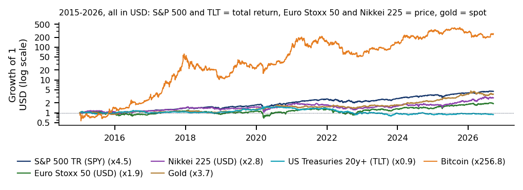
A comparison across asset classes is meaningful only on a single window. Each asset is therefore measured from 2 January 2015 to 18 September 2026; with different windows the comparison would mix different shocks, for example the 2008 crisis for one asset and not for another. All series are in US dollars (USD), except the EUR/RON exchange rate. TR (Total Return, with dividends or coupons reinvested) denotes a total-return series, with dividends or coupons reinvested, and TLT (iShares 20+ Year Treasury Bond ETF) is the exchange-traded fund (ETF) that holds US Treasury bonds with more than 20 years to maturity.
The chart places each asset in the risk–return plane. The vertical axis is the compound annual growth rate (CAGR), the growth an investor actually realised over the window. The horizontal axis is the annualised volatility on a logarithmic scale, so that the distance from 2% to 4% looks the same as that from 20% to 40%; without the log scale, Bitcoin would push all other assets into one corner.
The section asks two questions of this chart:
A descriptive one: which return and which risk each class delivered.
An inferential one: whether any difference between the classes is statistically significant, or whether the ordering on the chart is compatible with equal expected returns.
The interactive chart starts the common window on 2 January of the year chosen with the slider, from 2015 to 2024, and the list selects the asset whose figures are described below the chart. The ▶ button moves the start of the window forward one year at a time.
Question for the room On common dates in 2015–2026, the annualised difference in mean simple returns, SPY minus gold, is 1.9 pp, with an SE of 6.8 pp. Is it significant in a two-sided test at 5%?
Answer
We calculate t = 1.9/6.8 ≈ 0.28. We do not reject equal means; we do not establish that the means are equal. The test uses simple returns, not the difference between the plotted CAGRs (13.7% and 11.8%). For a single asset the standard error of the annualised mean return, σ/√Y with Y = 11.7 years, is 5.1 pp for the S&P 500 and 4.8 pp for gold. Under iid returns, with the same annual volatility and time span, more frequent sampling does not reduce the SE of the annualised mean.
Moving the start of the window changes the position of every asset on the chart. A ranking that changes with the start date of the sample is a property of the window rather than of the assets.
In brief
This section answers
what return and what risk did the main asset classes deliver?
is any difference between them statistically significant?
One window for every asset, 2 Jan 2015 – 18 Sep 2026
different windows would compare different shocks
Vertical axis: CAGR, the realised compound growth
Horizontal axis: annualised volatility on a log scale
2% to 4% looks as wide as 20% to 40%
All in USD (US dollar), except EUR/RON
TR: total return
TLT: the ETF of US Treasuries with more than 20 years to maturity
Over the full window, the S&P 500 with dividends has a CAGR of 13.7% and an annualised volatility of 17.6%. Gold has a CAGR of 11.8% and a volatility of 16.3%, computed on weekday quotes, and Bitcoin a CAGR of 60.6% with a volatility of 66.7%.
The series are not all equivalent investments. SPY and TLT include dividends and coupons, whereas the Euro Stoxx 50 and the Nikkei 225 are price indices, without dividends; a comparison with them is therefore not a test between total returns of equivalent investments. Ethereum, with a shorter sample, and the exchange rates EUR/USD and EUR/RON appear on the chart but are not tested. The "return" of an exchange rate omits the interest earned on the currency, which an investor holding that currency would receive.
The tests that follow concern the arithmetic mean of the returns and the Sharpe ratio, not the CAGR. The arithmetic mean is the parameter whose standard error has a simple form, and the Sharpe ratio is the risk-adjusted measure used to compare assets with different volatilities.
The precision of each point on the chart follows from the standard error (SE) of the annualised mean return. Under independent and identically distributed (iid) returns with annual volatility \(\sigma_A\), observed over \(Y\) years,
and the SE depends on the length of the sample in years, not on the number of observations. With \(Y = 11.7\),(0.10) gives 5.1 percentage points (pp) for the S&P 500 with dividends, 4.8 pp for gold, 6.0 pp for the Euro Stoxx 50, 6.2 pp for the Nikkei 225 and 19.4 pp for Bitcoin. Differences of a few points between the mean returns of the traditional assets are therefore within one standard error.
A difference between two assets must be tested directly, on the days when both are observed. The S&P 500 minus gold difference is \(+1.9\) pp a year, with an SE of 6.8 pp and \(t = 0.28\), far from any conventional critical value. The Sharpe ratios, each with an SE of about 0.29, are 1.05 for Bitcoin, 0.82 for the S&P 500, 0.76 for gold, 0.53 for the Nikkei 225, 0.37 for the Euro Stoxx 50 and 0.00 for TLT. This SE requires a finite fourth moment of returns, an assumption that Chapter 1 questions.
Overlapping confidence intervals do not test a difference, because the two estimates are correlated. The correct procedure bootstraps the paired difference of the two Sharpe ratios on common days. For the S&P 500 minus gold the difference is \(+0.06\), with a 95% interval of \([-0.65,\ +0.88]\). For the S&P 500 minus the Euro Stoxx 50 it is \(+0.46\), with an interval of \([0.09,\ 0.85]\), which is significant as a single test. Among the five non-crypto assets, however, there are \(\binom{5}{2} = 10\) pairs. With the Bonferroni correction each test is carried out at \(5\%/10 = 0.5\%\), and none of the ten differences survives.
An interval that contains zero does not show that the two Sharpe ratios are equal: the S&P 500 minus gold interval is compatible with gold ahead by 0.65 and with the S&P 500 ahead by 0.88. The comparison is inconclusive, and the risk–return chart describes the sample without ranking expected returns.
In brief
SE of the annualised mean return, \(\sigma_A/\sqrt{Y}\) with \(Y = 11.7\)
Volatility measures the dispersion of returns but not the path an investor lives through. The drawdown measures the latter: \(DD_t\) is the percentage by which the level at date \(t\) lies below its running peak, the highest level reached up to \(t\), and the maximum drawdown (MDD) is its most negative value over the sample.
The chart has two panels. The upper panel shows the level of the S&P 500 price index on a logarithmic scale, so that equal vertical distances represent equal percentage changes. The bar marks the 5.5 years needed to regain the peak of October 2007. The lower panel shows the drawdown \(DD_t\), in percent below the running peak; the index is at a new high whenever the curve touches zero.
In the interactive chart, the slider moves the end of the sample and the ▶ button replays the history day by day, so that each drawdown appears as it was lived, without knowledge of the recovery.
Question for the room The S&P 500 fell from 1,565.15 (9 October 2007) to 676.53 (9 March 2009). What percentage gain from the trough was needed to regain the peak?
Answer
(1,565.15/676.53 − 1) × 100 = 131.3%. The 56.8% decline uses the peak as its base; recovery uses the trough. The final level is 231.3% of the trough, so the gain is 131.3%. The recovery took 5.5 years from the peak, until 28 March 2013.
The depth of a fall and the gain needed to recover it are not symmetric. From the peak of 1,565.15 on 9 October 2007 to the trough of 676.53 on 9 March 2009 the index lost 56.8%, but regaining the peak required a gain of \((1{,}565.15/676.53 - 1) = 131.3\%\) from the trough: the loss is measured from the peak, the recovery from the trough.
In brief
Upper panel: the S&P 500 level (price index), log scale
the bar: 5.5 years to regain the October 2007 peak
Lower panel: the drawdown \(DD_t\), in % below the running peak
Since 2000 the S&P 500 has had four deep troughs. The dot-com crash reached \(-49\%\) in October 2002. The global financial crisis reached \(-57\%\) in March 2009, from 1,565.15 to 676.53 points, and the peak was regained only in March 2013. The COVID-19 fall, \(-34\%\) in March 2020, was the fastest of the four, and the inflation shock of 2022 reached \(-25\%\) in October 2022.
The four episodes differ in depth, speed and duration, and no single volatility number summarises them. The MDD is a path statistic: it can only deepen as the sample grows longer, since a longer sample contains more opportunities for a deep fall. MDDs of different assets or strategies must therefore be compared over the same horizon; the dependence on sample length is shown in the Appendix.
In brief
Four S&P 500 troughs since 2000
dot-com: \(-49\%\) (Oct 2002)
global financial crisis: \(-57\%\) (Mar 2009), from 1 565.15 to 676.53, regained only in Mar 2013
COVID-19: \(-34\%\) (Mar 2020), the fastest fall
inflation shock: \(-25\%\) (Oct 2022)
The MDD deepens with the sample length, so compare MDDs over the same horizon (Appendix)
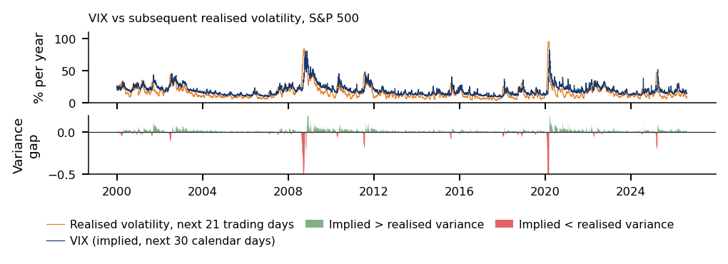
The volatility used so far is realised, computed from past returns. The VIX (CBOE Volatility Index, published by the Chicago Board Options Exchange) measures instead the volatility of the S&P 500 over the next 30 days that is implied by the prices of index options, in percent per year. It is a forward-looking quantity, priced by the market.
Since 2000 the VIX has been below 20 on 62% of the days and above 30 on 9% of them. The highest values are 82.7 on 16 March 2020, 80.9 on 20 November 2008 and 52.3 on 8 April 2025. The distribution is strongly skewed: long calm periods alternate with short episodes of intense stress. Volatility thus comes in regimes, which the GARCH models of Chapter 5 and the realised-volatility models of Chapter 9 describe.
The VIX exceeded the volatility realised over the next 21 trading days on 83% of the days. Ex post, the gap between implied and realised volatility contains two components: the variance risk premium, which option buyers pay for protection, and the forecast error. The premium is defined on variances, not as a difference of volatilities; the Appendix gives the definition.
In the interactive chart, two sliders set a lower and an upper threshold, and the chart reports the share of days with the VIX below the first and above the second. The ▶ button moves the thresholds step by step.
Question for the room What is the smallest integer threshold with at least 50% of the sample’s daily VIX values strictly below it? Check by moving the lower threshold.
Answer
45.4% of observations are below 17, and 51.4% are below 18. The required threshold is therefore 18. The median is 17.75; rounding it down does not give the required threshold. The mean, 19.79, is more sensitive to large extreme values. The VIX was below 20 on 62% of the days and at least 30 on 9%. The highest values are 82.7 on 16 March 2020, 80.9 on 20 November 2008 and 52.3 on 8 April 2025: calm periods are long, stress periods short and intense.
The threshold that splits the sample into two halves is close to the median, 17.75, and lies below the mean, 19.79. A mean above the median is the signature of a right-skewed distribution: a few days of extreme stress raise the mean, while most days are calm.
In brief
VIX: the S&P 500 volatility over the next 30 days implied by option prices
VIX: CBOE Volatility Index; CBOE: Chicago Board Options Exchange; in % per year
Since 2000: below 20 on 62% of days, above 30 on 9%
peaks 82.7 (16 Mar 2020), 80.9 (20 Nov 2008), 52.3 (8 Apr 2025)
Diversification depends on correlations, and the correlations between asset classes are not constant. The chart shows rolling correlations of daily log returns over windows of 252 trading days, about one calendar year. The prices are first joined on the days common to both assets; otherwise a return computed over a holiday of one market would be paired with a one-day return of the other.
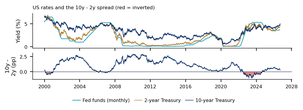
Between stocks and long-term Treasuries, through TLT, the mean rolling correlation was \(-0.43\) in 2010–2020 and \(+0.08\) in 2022–2026. Over the first period long bonds hedged equity losses; over the second the hedge disappeared. Between stocks and Bitcoin the mean rolling correlation rose from 0.01 in 2016–2019 to 0.38 in 2022–2026, as Bitcoin came to move more with risky assets.
Portfolio models that assume a fixed correlation miss such shifts; Chapter 4 and Chapter 6 treat time-varying dependence. Two traps affect crypto–equity correlations in particular. Asynchronous closes arise because crypto assets trade around the clock while exchanges close at fixed times (Appendix). The volatility bias arises because a correlation estimated in a turbulent period is mechanically higher even when the underlying dependence is unchanged (Appendix). Whether the stock–bond change is statistically significant is tested in Further Topics.
In the interactive chart, the slider sets the length of the rolling window from 63 to 756 trading days, and the ▶ button lengthens it step by step.
Question for the room The mean 252-day rolling correlation between the S&P 500 and TLT was −0.43 in 2010–2020 and +0.08 in 2022–2026. The ▶ button lengthens the window up to 756 days. What happens to the 2022–2026 mean?
Answer
It stays close to zero: +0.10 with the 63-day window, +0.08 with 252 and −0.02 with 756, while the 2010–2020 mean stays between −0.42 and −0.44. The change does not come from the window: since 2022, TLT no longer gains, on average, on the days when stocks lose. Computed directly on each subperiod, the correlation is −0.47 and +0.11. The S&P 500–Bitcoin correlation rose from 0.01 (2016–2019) to 0.38 (2022–2026).
The 2022–2026 mean stays close to zero for every window: \(+0.10\) with 63 days, \(+0.08\) with 252 and \(-0.02\) with 756, while the 2010–2020 mean stays between \(-0.42\) and \(-0.44\). The change is therefore not an artefact of the window length; computed directly on each subperiod, the stock–bond correlation is \(-0.47\) and \(+0.11\).
In brief
252-day rolling correlations of daily log returns, prices joined on common days first
Stocks vs long Treasuries: mean rolling \(-0.43\) (2010–2020), \(+0.08\) (2022–2026)
Stocks vs Bitcoin: mean rolling 0.01 (2016–2019), 0.38 (2022–2026)
Fixed-correlation portfolio models miss such shifts (Chapters 4 and 6)
Over 2015–2026 the asset classes delivered very different returns and risks, yet no ranking among the traditional assets survives a test of the paired difference corrected for multiple comparisons. The crises of 2000–2026 differ in depth and duration, volatility alternates between long calm periods and short stress, and the stock–bond correlation, on which much of diversification rests, changed sign after 2020.
The Romanian Market
This background section applies the same measurements to the Romanian market: the Bucharest Stock Exchange (BVB, Bursa de Valori București), its benchmark index BET and its long recovery after 2007.
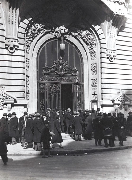
The Bucharest Stock Exchange opened in 1882, was closed in 1948 and was re-established in 1995; its history is in the Appendix. Its benchmark index, the BET (Bucharest Exchange Trading index), tracks the most traded Romanian companies. It was launched on 19 September 1997 at 1,000 points and is a price index; BET-TR is its total-return version, with dividends reinvested.
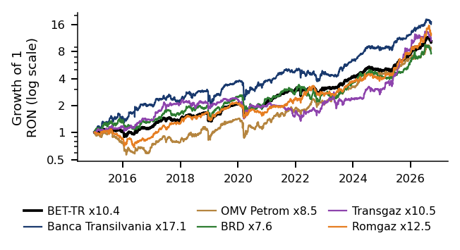
The largest listed companies are banks (Banca Transilvania and BRD), energy companies (OMV Petrom, Romgaz and Hidroelectrica) and utilities (Transgaz). Since September 2020 FTSE (Financial Times Stock Exchange, FTSE Russell, index provider) Russell has classified Romania as a Secondary Emerging market (FTSE Russell, 2026). The initial public offering (IPO) of Hidroelectrica, in July 2023, raised EUR 1.9 billion and is the largest in the exchange's history. TVBETETF (Patria-TVBETETF, the BVB-listed ETF on the BET index) is an ETF listed on the BVB that replicates the BET.
A market with a small number of large issuers, concentrated in banking and energy, has an index whose risk depends heavily on a few sectors. The same measurements used for the US market, CAGR, volatility and drawdown, show how this structure translates into the history of the index.
In brief
This background section answers
what do the same measurements show on the Romanian market?
BVB (Bursa de Valori București, the Bucharest Stock Exchange) (Appendix)
opened in 1882, closed in 1948, re-established in 1995
BET (Bucharest Exchange Trading index): the most traded Romanian companies (BVB (indices))
launched on 19 Sep 1997 at 1 000 points
BET-TR: its total-return version, with reinvested dividends
Largest companies
banks (Banca Transilvania, BRD), energy (OMV Petrom, Romgaz, Hidroelectrica), utilities (Transgaz)
Classified as Secondary Emerging by FTSE Russell (FTSE: Financial Times Stock Exchange), the index provider, since September 2020 (FTSE Russell (2026))
Hidroelectrica: the largest IPO in BVB (Bursa de Valori București, the Bucharest Stock Exchange) history, EUR 1.9 bn, July 2023 (BVB (history))
The chart shows the official closing values of the BET on a logarithmic scale. From the peak of 24 July 2007 to the trough of 25 February 2009 the index fell by 82.5%, much more than the S&P 500 in the same crisis. On 19 December 2018 the index lost 11.2% in a single day, after the announcement of a tax on bank assets, an event studied in Further Topics.
The interactive chart lets the start date of the sample move between 1 January 1997 and 1 January 2025 with the slider; the ▶ button moves it one year at a time, and the chart recomputes the growth and the drawdowns from the chosen start.
Question for the room How long did the BET take to regain its peak of 24 July 2007?
Answer
13.6 years elapsed between the peak on 24 July 2007 and recovery on 16 March 2021. The index fell by 82.5% to the trough on 25 February 2009; the 12.1-year interval runs from this trough to the recovery. The 5.5-year interval refers to recovery of the S&P 500’s 2007 peak. Over the whole of 1997–2026 the BET grew 32.8 times, a CAGR of 12.8%.
The BET regained its 2007 peak only on 16 March 2021, 13.6 years later, compared with 5.5 years for the S&P 500. On 18 September 2026 the index was 32.8 times its launch value, a CAGR of 12.8% over 29 years. A high long-run growth rate and a recovery of more than a decade coexist in the same series: the CAGR summarises the endpoints, the drawdown the path between them.
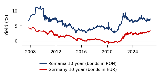
The Romanian series since 2015 are in the Appendix: BVB equities with dividends (Appendix), the EUR/RON exchange rate (Appendix) and Romanian versus German government bond yields (Appendix).
In brief
Official closing values, log scale
from the peak of 24 Jul 2007 to the trough of 25 Feb 2009: \(-82.5\%\)
regained only on 16 Mar 2021, after 13.6 years
19 Dec 2018: \(-11.2\%\) in one day, after the bank-tax announcement
18 Sep 2026: \(\times 32.8\) since launch, CAGR 12.8% over 29 years
Crypto assets and stablecoins appear throughout the course data. This background section defines them and asks what their prices measure: Bitcoin and Ethereum are traded assets with their own risk, whereas a stablecoin is designed to keep a fixed value, and the question is how well it does so.
On 31 October 2008 a paper signed with the pseudonym Satoshi Nakamoto, Bitcoin: A Peer-to-Peer Electronic Cash System, proposed an electronic currency without a trusted intermediary (Nakamoto, 2008). The record of transactions is a blockchain: a shared ledger, copied on many computers and extended block by block, in which every participant can verify the history.
Bitcoin, launched in 2009, has a fixed supply rule, with at most 21 million coins. Its security rests on proof of work: adding a block costs computing power, so rewriting the history of transactions would require repeating that work and is expensive.
Ethereum is a blockchain that runs programs, called smart contracts, and its coin is Ether. A token is a unit recorded on a blockchain that represents a coin, a claim or a right; it may stand for a currency, a share of a fund or access to a service.
The statistical properties, pricing and regulation of crypto assets are surveyed by Härdle, Harvey & Reule (2020).Liu & Tsyvinski (2021) find that cryptocurrency returns have low exposures to stock, currency and commodity factors and are explained instead by crypto-specific factors, momentum and investor attention. Pele et al. (2023) show that tail, memory and moment factors set cryptocurrencies apart from other asset classes.
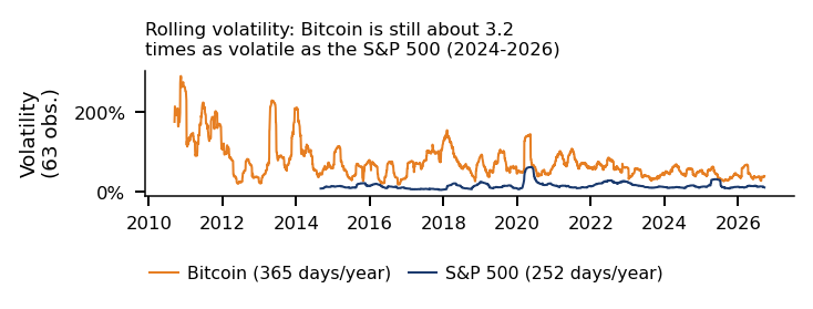
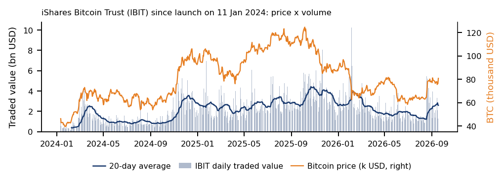
In 2024–2026 Bitcoin was still about 3.2 times as volatile as the S&P 500 (Appendix). Since January 2024 spot Bitcoin ETFs trade in the US (Appendix); how an ETF works is the subject of the next section.
In brief
Ethereum: a blockchain that runs programs (smart contracts)
its coin is Ether
A token is a unit on a blockchain representing a coin, a claim or a right
Question for the room On what proportion of observed days in 2019–2026 is the daily USDT (Tether, a US dollar stablecoin) quote in the data within 0.5% of USD 1?
Answer
The proportion is 93.0%. The 98% figure corresponds to the wider ±1% band; about 7% is the proportion outside the ±0.5% band. The calculation uses the available daily quotes and does not describe all intraday movements. The extreme deviations are from March 2020: 1.054 USD on 12 March and 0.974 USD on 18 March.
A stablecoin is a token designed to keep a fixed value, the peg, usually 1 USD. There are two main designs. A reserve-backed stablecoin holds cash and short-term Treasury bills (T-bills) and is redeemable at 1 USD; an algorithmic stablecoin relies instead on a second token and on trading rules that are supposed to restore the peg.
A depeg occurs when the price leaves the peg. The algorithmic TerraUSD lost its peg and collapsed in May 2022, showing that a design without reserves can fail when holders all try to exit at once. For a reserve-backed coin, the deviation from the peg measures the market's confidence in the reserves and in the redemption mechanism.
In brief
Stablecoin: a token designed to keep a fixed value (peg), usually 1 USD
reserve-backed (cash, short-term T-bills) and redeemable at 1 USD, or algorithmic (a second token and trading rules)
Depeg: the price leaves the peg
the algorithmic TerraUSD lost its peg and collapsed in May 2022
The chart shows the price of Tether (USDT) minus 1 USD, in percent. The dashed lines mark the bands of \(\pm 0.5\%\) and \(\pm 1\%\) around the peg, and the inset enlarges March 2020, when the deviations were largest. In the interactive chart, the slider sets the width of the band around the peg and the list selects the period, the whole of 2019–2026, March 2020 or a single year.
Over 2019–2026 USDT stayed within \(\pm 0.5\%\) of 1 USD on 93% of the observed days and within \(\pm 1\%\) on 98% of them. The figures use the available daily quotes and do not describe intraday movements; the extreme deviations, in March 2020, were 1.054 USD on 12 March and 0.974 USD on 18 March.
The supply of a stablecoin is not its peg (Appendix). The circulating value can fall, as holders redeem, while the price stays at 1 USD. Tokenisation of other assets and the regulation of digital assets are discussed in the Appendix.
Index funds and ETFs now hold a large part of the equity market. This background section explains how an ETF keeps its price close to the value of its assets and what capitalisation weighting implies for an investor who buys the index, before the case study asks what the growth of passive investing does to prices.
Most ETFs are passive: they replicate an index at low cost. Their shares trade on an exchange throughout the day, while the value of the fund is computed once a day as the net asset value (NAV), the fund's assets minus its liabilities, per share. Nothing in ordinary trading forces the market price of an ETF share to equal the NAV.
The link is provided by authorised participants (APs), large dealers allowed to deal directly with the ETF issuer. In a creation, the AP delivers the basket of underlying assets to the issuer and receives new ETF shares; in a redemption, it returns ETF shares and receives the basket. When the ETF trades above its NAV, an AP can buy the basket, create shares and sell them on the exchange; when it trades below, the AP buys shares, redeems them and sells the basket. This arbitrage keeps the market price close to the NAV; a worked example is in Further Topics.
The diagram shows the flows: the AP exchanges the basket for ETF shares with the issuer and trades the shares with investors on the exchange.
An index of \(n\) stocks can weight its constituents in two simple ways. With capitalisation weights, \(w_i = MC_i/\sum_{j=1}^{n} MC_j\), where \(MC_i\) is the market capitalisation of stock \(i\), its price times the number of shares. With equal weights, \(w_i = 1/n\), rebalanced periodically. A cap-weighted index needs no rebalancing, since the weights move with prices; an equal-weighted index must sell winners and buy losers to return to \(1/n\).
The concentration of the weights is measured by the effective number of holdings, the inverse of the Herfindahl index:
For equal weights (0.11) gives \(N_{\text{eff}} = n\), and if one stock holds all the weight it gives 1. When a few firms dominate, \(N_{\text{eff}}\) is far smaller than \(n\). The measure uses only the weights: the diversification of risk also depends on the covariances of the returns, which (0.11) ignores.
A cap-weighted index is therefore more concentrated than its number of stocks suggests, and the passive funds that track it carry the concentration of its largest firms. Concentration returns in Chapter 3, Chapter 4 and Chapter 17.
In brief
Definition (Index weights and weight concentration).
Capitalisation weights: \(w_i = MC_i/\sum_{j=1}^{n} MC_j\), with \(n\) stocks in the index
\(MC_i\): the market capitalisation of stock \(i\), price \(\times\) number of shares
Two ETFs on the same 500 stocks allow a direct comparison of the two weighting schemes. SPY tracks the S&P 500 with capitalisation weights. RSP, the Invesco S&P 500 Equal Weight ETF, holds the same stocks, each with weight \(1/500\), rebalanced periodically. Both are measured with adjusted prices, that is, as total returns.
The chart has two panels. The left panel shows the value of 1 USD invested in each ETF in April 2003, when RSP was launched, on a log scale. The right panel shows the ratio SPY/RSP, equal to 1 in April 2003: the ratio rises when cap weights do better and falls when equal weights do better. In the interactive chart, the slider moves the start year from 2003 to 2025, and both series are rebased to 1 at the new start.
Question for the room Keep the sample end fixed and move the start from April 2003 to January 2015. Both series are rebased to 1 at the new start. Approximately what does the final SPY/RSP ratio become?
Answer
The final ratio becomes 1.396, approximately 1.40. The value 1.07 corresponds to an April 2003 start; 1.31 corresponds to a January 2023 start. Rebasing changes the final ratio because it changes the comparison base. The conclusion depends on the end date, though: the ratio, equal to 1 in April 2003, had fallen to 0.76 in April 2015, and the SPY advantage comes from the 31% rise of the ratio since January 2023. A higher realised return does not show an expected premium.
Moving the start changes the conclusion. With an April 2003 start the final ratio is 1.07; with a January 2015 start it is about 1.40, and with a January 2023 start 1.31. The ratio, equal to 1 in April 2003, had fallen to 0.76 by April 2015: equal weights led for more than a decade, and the advantage of SPY over the whole sample comes from the years after 2023.
In brief
The chart
left: the value of 1 USD invested in April 2003, log scale
right: the SPY/RSP ratio, equal to 1 in April 2003
Measured as total returns from RSP's launch in April 2003, SPY multiplied the initial investment by 12.7 and RSP by 11.9, so the ratio ends at 1.07. Over more than two decades the two weighting schemes delivered similar wealth.
The ratio SPY/RSP has risen by 31% since January 2023, when a handful of very large companies drove the index. The ratio measures relative performance: it shows that the largest firms outperformed the average firm, but it is not a direct measure of concentration or of passive ownership. Concentration requires the weights, as in (0.11), and passive ownership requires holdings data, which the case study uses.
In brief
Total return (adjusted close) since RSP's launch in April 2003
SPY \(\times 12.7\), RSP \(\times 11.9\); the ratio ends at 1.07
SPY/RSP rose by 31% since January 2023
a handful of very large companies drove the index
The ratio measures relative performance
it is not a direct measure of concentration or of passive ownership
An ETF tracks its index through creation and redemption by authorised participants. A cap-weighted index is more concentrated than its number of stocks suggests, and the passive funds that track it inherit that concentration. Cap and equal weights delivered similar wealth since 2003, and the recent advantage of cap weights is a feature of the window that starts in 2023.
Case Studies: Stock Market Competition and Treasury Bond Risk
The section presents two recent papers that use the chapter's measurements on questions of current interest:
Haddad, Huebner & Loualiche (2025) asks whether the growth of passive investing makes stock prices less elastic, once the reaction of the remaining active investors is taken into account.
Pflueger (2025) asks when US Treasury bonds hedge an equity portfolio, and the course data extend its evidence to September 2026.
Case Study: What Happens When Passive Investing Grows? (1/2)
Haddad, Huebner & Loualiche (2025), published in the American Economic Review 115(3), 975–1018, study the effect of passive investing on prices. Their question is whether, when some investors turn passive, the others trade more aggressively and undo the effect on prices.
The central quantity is the demand elasticity\(\mathcal{E}_i\) of investor \(i\): the percentage fall in the number of shares the investor demands after a 1% rise in the price. An active investor who buys when a stock is cheap and sells when it is expensive has a positive elasticity. A passive investor holds the index weights whatever the price and has \(\mathcal{E}_i = 0\). The paper asks how the elasticity of the whole market changes when investors move from the first group to the second.
In brief
This section asks
what does a landmark paper find about the effect of passive investing on prices?
The aggregate elasticity\(\mathcal{E}_{agg}\) is the holdings-weighted average of the individual elasticities \(\mathcal{E}_i\) (the paper's eq. 2). It determines how a demand shock moves the price:
\[\Delta p = \mathcal{E}_{agg}^{-1}\,\Delta\bar d,\]
(0.12)
the paper's eq. (3), where \(\Delta\bar d\) is the average demand shock, the percentage change in the shares demanded at the old price, and \(\Delta p\) is the change in the log price.
By (0.12), a lower aggregate elasticity lets the same demand shock move the price more. Prices become more volatile, and, since the price reacts more to flows that carry no information, less informative (the paper's Section II.A). The mechanism is consistent with the evidence of Ben-David, Franzoni & Moussawi (2018) that stocks with higher ETF ownership are more volatile.
In brief
Aggregate elasticity\(\mathcal{E}_{agg}\): the holdings-weighted average of the \(\mathcal{E}_i\) (eq. 2)
\[ \Delta p = \mathcal{E}_{agg}^{-1}\,\Delta\bar d \quad \text{(eq.\ 3)} \]
\(\Delta\bar d\): the average demand shock, the percentage change in the shares demanded at the old price
\(\Delta p\): the change in the log price
a lower \(\mathcal{E}_{agg}\) lets the same shock move the price more: prices more volatile and less informative (Section II.A)
The paper allows the remaining active investors to react. The strategic response\(\chi\) enters each investor's elasticity as \(\mathcal{E}_i = \bar{\mathcal{E}}_i - \chi\,\mathcal{E}_{agg}\) (eq. 4), where \(\bar{\mathcal{E}}_i\) is the investor's own component. When the market as a whole becomes less elastic, each active investor becomes more elastic. With \(\chi = 0\) nobody reacts; as \(\chi \to \infty\) the others fully offset any change.
If a share \(1-\alpha\) of holdings turns passive, where \(\alpha\) is the share still active, the aggregate elasticity relative to the all-active market (\(\alpha = 1\)), with the same own elasticities, is
the paper's eq. (5); its derivation is in Further Topics. The first term, \(\alpha\), is the direct fall: the passive investors' elasticity drops out. The second term is the part offset by the active investors' response; it is 0 when \(\chi = 0\).
The slide's question takes 30% of investors turning passive, \(\alpha = 0.7\), with no reaction, \(\chi = 0\), and asks what share of the aggregate elasticity is left.
The chart plots (0.13). The horizontal axis is the share of investors turned passive, \(1-\alpha\), and the vertical axis the aggregate elasticity relative to the all-active market; each curve corresponds to one value of \(\chi\). In the interactive chart, one slider sets the strategic response \(\chi\) between 0 and 10 and the other the share turned passive; the ▶ button raises \(\chi\) step by step.
Question for the room 30% of investors turn passive (α = 0.7). The ▶ button raises the strategic response χ up to 10. How does the pass-through rate 1/(1 + χα) change as χ rises?
Answer
It falls from 1.00 (χ = 0) to 0.32 (χ = 2.97, the paper's estimate) and to 0.13 (χ = 10): active investors offset a growing part of each move to passive management. The pass-through rate is not the active share α. The aggregate elasticity left, eq. (5), is 0.70 with χ = 0, 0.90 with χ = 2.97, so two-thirds of the fall is offset, and 0.96 with χ = 10.
With no reaction, \(\chi = 0\),(0.13) gives 0.70: the aggregate elasticity falls in proportion to the share that turned passive. With the paper's estimate, \(\chi = 2.97\), 0.90 is left, so two-thirds of the fall is offset by the active investors; with \(\chi = 10\), 0.96 is left. At 100% passive all curves reach 0, whatever \(\chi\): nobody is left to absorb shocks.
The pass-through rate \(1/(1+\chi\alpha)\), introduced two slides later, falls as \(\chi\) rises: at \(\alpha = 0.7\) it is 1.00 for \(\chi = 0\), 0.32 for \(\chi = 2.97\) and 0.13 for \(\chi = 10\).
In brief
Horizontal axis: the share of investors turned passive, \(1-\alpha\)
Vertical axis: \(\mathcal{E}_{agg}\) relative to the all-active market, eq. (5)
Answer: 0.70 if nobody reacts (\(\chi = 0\))
With the paper's \(\chi = 2.97\), 0.90 is left
two-thirds of the fall is offset
With \(\chi = 10\), the aggregate elasticity left is 0.96
The data are the quarterly holdings of US institutional managers from Form 13F, filed with the Securities and Exchange Commission (SEC), over 2001–2020. They cover about 80% of US market capitalisation.
The estimated strategic response is \(\chi = 2.97\), with an SE of 0.47 (the paper's Table 2, row 1), which gives a 95% interval of about \([2.0,\ 3.9]\). Investors do react: the estimate is far both from 0, no reaction, and from \(\infty\), full offset.
The result supports a causal reading, conditional on the paper's identifying assumption (Theorem 1): the same investor meets a different mix of other investors in each stock. This variation across stocks separates the investor's own elasticity from its response to the others. The instruments, the generalised method of moments (GMM) estimator and the demand system are described in Appendix.
In brief
Data: quarterly holdings of US institutional managers from Form 13F, 2001–2020
Form 13F: filed with the SEC (Securities and Exchange Commission)
In the paper's data the median active share fell from 81.4% in 2001 to 59.5% in 2020, a log change of \(\ln(81.4/59.5) = 31.3\%\). The question is how much of this fall passes into the aggregate elasticity.
The answer is the pass-through (the paper's eq. 28), the percentage change in \(\mathcal{E}_{agg}\) per 1% change in the active share \(\alpha\):
where \(\alpha = 0.68\) is the time average of the active share in the paper (p. 1006). The pass-through depends on \(\alpha\): it is 0.29 at \(\alpha = 0.814\) (2001) and 0.36 at \(\alpha = 0.595\) (2020).
Combining the two figures, stocks became about \(0.33 \times 31.3\% \approx 10\%\) less elastic over 2001–2020; the paper's abstract reports 11%. Without the strategic response the fall would have been the full 31.3%. Inelastic stocks are, in the paper's Table 5, more volatile and less liquid; robustness and reduced-form checks are in Appendix.
In brief
Implication: the median active share fell from 81.4% (2001) to 59.5% (2020)
i.e. \(\ln(81.4/59.5) = 31.3\%\)
Pass-through (eq. 28): the % change in \(\mathcal{E}_{agg}\) per 1% change in \(\alpha\)
The model imposes one strategic response \(\chi\) for all investors and has no fund flows (the paper's Section I.B). Investors who differ in how strongly they react, or flows that move with prices, would change the offset; all the stated limits, and what the course data can check, are listed in Appendix.
An open question is whether passive investing changes price formation itself. Sammon (2025) finds that higher passive ownership makes prices anticipate earnings announcements less. Passive ownership is, however, endogenous, so a correlation between passive ownership and price informativeness is not by itself a causal effect.
The slide's question takes the paper's \(\chi = 2.97\) and an active share of \(\alpha = 0.5\). By (0.14) the pass-through is \(1/(1 + 2.97 \times 0.5) = 0.40\), larger than at \(\alpha = 0.68\): with fewer active investors left, fewer remain to offset each further switch to passive.
In brief
One limitation: one \(\chi\) for all investors, with no fund flows (Section I.B)
all stated limits and what the course data can check: Appendix
Open question: does passive investing change price formation?
Sammon (2025): higher passive ownership makes prices anticipate earnings announcements less
passive ownership is, however, endogenous: it depends on firm characteristics, so the link need not be causal
Question for the room: with \(\chi = 2.97\), what pass-through would an active share of \(\alpha = 0.5\) imply?
why is it larger than at \(\alpha = 0.68\)?
Answer: \(1/(1 + 2.97 \times 0.5) = 0.40\)
with fewer active investors left, there are fewer to offset each further switch to passive
The second case study asks when US Treasury bonds protect an equity portfolio. Pflueger (2025), published in the Journal of Financial Economics 167, 104027, measures the protection with the bond's stock market beta:
where \(r_b\) is the excess return on the 10-year Treasury bond and \(r_s\) the excess return on the US stock market. With \(\beta_b < 0\) the bond gains when stocks lose, so it hedges; with \(\beta_b > 0\) the bond loses together with stocks, so it is a risky asset.
The paper's claim is that the positive nominal bond beta of the 1980s required two conditions at once: volatile supply shocks and a monetary policy that reacts quickly and strongly to inflation. The mechanism is in the paper's model, presented two slides later.
In brief
The question: when do US Treasury bonds protect an equity portfolio?
The chart has two panels. The left panel shows the nominal \(\beta_b\) of (0.15) estimated over rolling windows of 20 quarters (5 years); the dotted lines mark 2001Q2 and 2020Q1, the breaks used below. The right panel shows daily \(\beta_b\) over 120-day windows for the nominal bond and for TIPS (Treasury Inflation-Protected Securities), the inflation-indexed US Treasury bonds. In the interactive chart, the two sliders set the quarterly and the daily window lengths, and the ▶ button changes them step by step.
Question for the room In the quarterly regression for 2001Q2–2019Q4, the beta of the 10-year nominal bond is −0.34. If the equity market’s excess return is 1 pp lower, how does the bond’s fitted excess return change?
Answer
The fitted change is (−0.34) × (−1 pp) = +0.34 pp. The negative sign (SE 0.06) indicates an opposite association during this subperiod; it does not guarantee a gain in every quarter with falling equities. The value 2.94 comes from incorrectly inverting the coefficient. In 1979Q4–2001Q1 the beta is 0.27. In 2020Q1–2026Q2 the nominal beta is 0.00 (SE 0.17) and the TIPS beta 0.19 (SE 0.13). On the daily returns of 2026 (up to 18 September) the nominal beta, 0.22, rises above the TIPS beta, 0.17; on the 120-day window of the chart the values on 18 September are 0.27 and 0.19.
On the course data the nominal \(\beta_b\) is 0.27 in 1979Q4–2001Q1 and \(-0.34\) in 2001Q2–2019Q4; the paper (NBER version, Table 2) reports 0.24 and \(-0.31\). The 5-year \(\beta_b\) turned positive again in 2023Q4 and is 0.26 in 2026Q2.
A beta is a regression coefficient: with \(\beta_b = -0.34\), a market excess return 1 pp lower is associated with a fitted bond excess return 0.34 pp higher. It describes an average association over the subperiod and does not guarantee a gain in every quarter in which equities fall.
In brief
Left: nominal \(\beta_b\) over rolling windows of 20 quarters (5 years); dotted lines at 2001Q2 and 2020Q1
Right: daily \(\beta_b\) over 120-day windows, for the nominal bond and for TIPS
TIPS (Treasury Inflation-Protected Securities): inflation-indexed US Treasury bonds
Nominal \(\beta_b\) on the course data: 0.27 in 1979Q4–2001Q1 and \(-0.34\) in 2001Q2–2019Q4
in the paper (NBER version, Table 2): 0.24 and \(-0.31\)
The 5-year \(\beta_b\) turned positive again in 2023Q4 and is 0.26 in 2026Q2
The paper's model is a three-equation New Keynesian model: the consumption Euler equation, the Phillips curve and the monetary policy rule. Preferences have habit formation, so risk premia vary over time. In the model a supply shock raises inflation and lowers output, stagflation, and nominal bonds then fall together with stocks.
The model is calibrated separately for 1979Q4–2001Q1 and 2001Q2–2019Q4. The 2001Q2 break is the date at which the correlation between inflation and the output gap, actual minus potential output, turns positive (Campbell, Pflueger & Viceira, 2020). Bond betas are not targeted in the calibration; the model reproduces them, which is the test of its explanation.
The course replication differs from the paper in its data. Bond returns come from the FRED constant-maturity yields (DGS10 for the nominal bond, DFII10 for TIPS), with duration fixed at 10 years, so that the quarterly return is approximated by \(r_b \approx -10\,\Delta y_t + y_t/4\), where \(y_t\) is the 10-year yield; the paper uses zero-coupon curves. Stock returns are the cap-weighted US market (CRSP, Center for Research in Security Prices) from the Kenneth French library, and SPY for daily data. Quarterly excess returns are measured over the 3-month T-bill, as in the paper. TIPS are used only from 2003, whereas the paper fills the earlier period with UK (United Kingdom) inflation-linked bonds, and the sample is extended to September 2026.
In brief
The paper's model: a three-equation New Keynesian model
the consumption Euler equation, the Phillips curve and the monetary policy rule
a supply shock raises inflation and lowers output (stagflation): nominal bonds fall together with stocks
Calibration: separately for 1979Q4–2001Q1 and 2001Q2–2019Q4
the 2001Q2 break: the correlation between inflation and the output gap (actual minus potential output) turns positive (Campbell, Pflueger & Viceira (2020))
bond betas are not targeted in the calibration; the model reproduces them
What the course replication does differently
bonds: FRED (Federal Reserve Economic Data) constant-maturity yields (DGS10, DFII10), duration fixed at 10 years
\(r_b \approx -10\,\Delta y_t + y_t/4\) per quarter, with \(y_t\) the 10-year yield; the paper uses zero-coupon curves
stocks: the cap-weighted US market (CRSP, Center for Research in Security Prices), from the Kenneth French library; daily, SPY
quarterly excess returns: over the 3-month Treasury bill (T-bill), as in the paper
TIPS only from 2003 (the paper fills the earlier period with UK inflation-linked bonds)
The course data reproduce the 2001 sign change. The nominal \(\beta_b\) is 0.27 (SE 0.14, 86 quarters) in 1979Q4–2001Q1 and \(-0.34\) (SE 0.06, 75 quarters) in 2001Q2–2019Q4. The explanation through supply shocks and monetary policy comes from the model; the regression alone does not identify it.
Over 2020Q1–2026Q2 the nominal \(\beta_b\) is 0.00 (SE 0.17) and the TIPS \(\beta_b\) 0.19 (SE 0.13). Since 11 March 2020 the daily nominal beta has been below the TIPS beta on 84% of the days. In the paper, a nominal beta below the real one signals little stagflation risk.
The evidence has limits. The 120-day windows are noisy, the bond duration is approximated, and the conclusion rests on one calibrated model.
In 2026, up to 18 September, the nominal \(\beta_b\) estimated on daily returns is 0.22 and the TIPS \(\beta_b\) 0.17. In the paper's reading, this ordering signals a rise in stagflation risk: the difference, 0.05 (SE 0.02), is positive for the first time in a calendar year since 2018. One partial year does not, however, show a return to the 1980s.
In brief
Type of evidence: replication (the 2001 sign change, reproduced on the course data)
nominal \(\beta_b\) 0.27 (SE 0.14, 86 quarters) in 1979Q4–2001Q1
nominal \(\beta_b\)\(-0.34\) (SE 0.06, 75 quarters) in 2001Q2–2019Q4
the explanation through supply shocks and monetary policy comes from the model; the regression alone does not identify it
since 11 March 2020 the daily nominal beta is below the TIPS beta on 84% of the days
in the paper, a nominal beta below the real one signals little stagflation risk
Limits
120-day windows are noisy
the bond duration is approximated
the conclusion rests on one calibrated model
Question for the room: in 2026 (up to 18 September) the nominal \(\beta_b\) estimated on daily returns is 0.22 and the TIPS \(\beta_b\) 0.17
what signal would the paper read in this ordering?
Answer: a rise in stagflation risk
the difference, 0.05 (SE 0.02), is positive for the first time in a calendar year since 2018
one partial year does not, however, show a return to the 1980s
Section summary
Haddad, Huebner & Loualiche (2025) estimate that active investors offset about two-thirds of the fall in elasticity caused by the move to passive investing, so stocks became about 10% less elastic over 2001–2020 instead of 31%. Pflueger (2025) explains the sign of the stock–bond beta by supply shocks and the monetary policy response; the course data reproduce the 2001 sign change, and since 2023 the 5-year beta has been positive again.
AI for Scientific Discovery
The section runs one pass of the AI-assisted research loop, introduced at the start of the chapter, on a new question suggested by the SPY–RSP comparison: is there a concentration premium? The pass shows what an assistant typically proposes, which checks must be fixed before the data are seen, and what the estimate supports.
Hypothesis: Is There a Concentration Premium? (1/2)
The SPY–RSP comparison of the previous sections is descriptive. It cannot identify the passive-ownership mechanism of the case study, since many forces move the relative performance of the largest firms.
A typical assistant proposal reads: "passive flows favour the largest firms, so cap weights beat equal weights." The claim names a mechanism and a prediction, but it offers no estimate, no interval and no rival explanation.
One pass of the discovery loop turns the proposal into a testable question. The literature step uses peer-reviewed papers, with every DOI resolved by the researcher. The hypothesis step states three competing explanations, passive flows, sector composition and the earnings growth of the largest firms, each with one implication the others do not share. The data-and-code step uses the adjusted, total-return prices of SPY and RSP, joined on common days.
In brief
This section asks
how does one pass of the AI-assisted research loop look on a new question?
The SPY–RSP comparison is descriptive
it cannot identify the case study's passive-ownership mechanism
A typical assistant proposal
“passive flows favour the largest firms, so cap weights beat equal weights”
Discovery loop in one pass
literature: peer-reviewed papers, every DOI resolved yourself
hypothesis: three competing explanations (passive flows, sector composition, earnings growth of the largest firms), each with one implication the others do not share
data and code: SPY and RSP adjusted (total-return) prices, joined on common days
Hypothesis: Is There a Concentration Premium? (2/2)
The test uses the daily spread \(d_t = r_{\mathrm{SPY},t} - r_{\mathrm{RSP},t}\), where \(r_{\mathrm{SPY},t}\) and \(r_{\mathrm{RSP},t}\) are the daily log returns of the two ETFs on day \(t\). The null hypothesis \(H_0: \mathbb{E}[d_t] = 0\), no premium, is tested against \(H_1: \mathbb{E}[d_t] \neq 0\), where \(\mathbb{E}[d_t]\) is the true mean daily spread.
The checks are fixed before the data are seen: the price type, the calendar join and the windows, the full sample and two halves. The statistic is
\[t = \frac{\bar d}{\operatorname{SE}(\bar d)},\]
(0.16)
with the Newey–West standard error, which is heteroskedasticity and autocorrelation consistent (HAC): it remains valid when \(d_t\) is autocorrelated or its variance changes over time. Its construction is in the Appendix. Fixing the windows in advance prevents choosing, after the fact, the period in which the spread looks largest.
The sample runs from May 2003 to September 2026, 5,884 trading days. The chart shows, for the full sample and for each half, the mean of \(d_t\) as a dot, its HAC 95% interval as a bar and, in red, \(\pm\) the minimum detectable effect (MDE). The MDE is the smallest true effect that a two-sided test at 5% detects with 80% power; for a test based on (0.16) it is about \(2.8 \times \operatorname{SE}\) (Appendix).
In the interactive chart, the slider moves the date that splits the sample into two halves, from 2005 to 2024, and the ▶ button moves it one year at a time; a second panel shows the cumulative spread.
Question for the room Over the full sample the mean SPY − RSP difference is +0.29% a year, with t = 0.27. Does this mean that there is no concentration premium?
Answer
No. The estimated mean is +0.29% a year, with an HAC SE of about 1.10 pp and t = 0.27. We do not reject a zero mean at 5%. The MDE of about 3.1% a year corresponds to approximately 80% power under the Normal approximation. Smaller effects have power below 80%, not necessarily below 50%. The p-value of about 0.79 is not the probability that the premium exists. The sign changes between the halves: −2.28% (t = −1.75) in 2003–2014 and +2.85% (t = 1.63) in 2015–2026.
Over the full sample the mean spread is \(+0.29\%\) a year, with \(t = 0.27\). In the halves fixed in advance it is \(-2.28\%\)(\(t = -1.75\)) from May 2003 to December 2014 and \(+2.85\%\)(\(t = 1.63\)) from January 2015 to September 2026. Every interval contains 0, and the sign flips between the halves: the "premium" is a feature of the chosen window.
"Not significant" is not "no effect". The full-sample MDE is 3.1% a year: the test had about 80% power against a premium of that size, and less against smaller ones. The p-value, about 0.79, is not the probability that a premium exists. What the result supports is description.
A natural next question is whether the SPY − RSP spread survives after controlling for sector returns. The project regresses \(d_t\) on the daily log returns of the SPDR sector ETFs and tests \(H_0\): intercept \(= 0\), with HAC standard errors. A nonzero intercept would be a spread not explained by the different sector weights of the two funds.
The regressors and the window are fixed before estimation. The main specification uses the nine Select Sector SPDRs launched in December 1998 (XLB, XLE, XLF, XLI, XLK, XLP, XLU, XLV and XLY), which cover the whole mini-case window. XLRE (real estate, 2015) and XLC (communication services, 2018) enter only a second, shorter specification, with its window reported.
The specification guards against two traps. A join that keeps only the days on which every regressor exists silently cuts the sample to 2018–2026 if XLC is included, and the intercept would then estimate the spread of a different period. RSP is rebalanced to equal weights each quarter, so its sector loadings are not exactly constant. The full workflow of the project is in Further Topics.
In brief
Question: does the SPY \(-\) RSP spread survive after controlling for sector returns?
regress \(d_t\) on the daily log returns of the SPDR sector ETFs
test \(H_0\): intercept \(= 0\) with HAC standard errors
Regressors and window, fixed before estimation
main specification: the nine Select Sector SPDRs launched in December 1998 (XLB, XLE, XLF, XLI, XLK, XLP, XLU, XLV, XLY), which cover the whole mini-case window
XLRE (real estate, 2015) and XLC (communication services, 2018) only in a second, shorter specification, with its window reported
A join that keeps only days on which every regressor exists silently cuts the sample
to 2018–2026 if XLC is included
the intercept would then estimate the spread of a different period
A comparison is trustworthy only with the right data, the right calendar and an honest interval. A "daily price" depends on the venue and on the observation time, and each series must be joined on common days before returns are compared.
Each wave of financial models solved a new problem with new data and computing power, without replacing the earlier ones, and bubbles and crashes have recurred for four centuries. The mean return and the Sharpe ratio are known only to the precision that the number of years allows; an interval that contains zero means "inconclusive", not "equal".
Cap-weighted passive investing carries the concentration of the market. A claim, whether made by a human or generated by AI, needs an estimate, an interval, a rival explanation and a stated limitation.
In brief
A comparison is trustworthy only with the right data, the right calendar and an honest interval
A “daily price” depends on the venue and on the observation time
Each wave of models solved a new problem with new data and computing power
without replacing the earlier ones
Bubbles and crashes have recurred for four centuries
The mean and the Sharpe ratio are known only to the precision the number of years allows
an interval that contains zero means “inconclusive”, not “equal”
The retrieval questions return to the chapter's main results: the precision of a mean, the calendar join, the reading of an interval and the meaning of the SPY/RSP ratio.
The second group introduces Chapter 1, which asks how heavy the tails of daily returns are, whether volatility has long memory and at which horizon returns approach the Normal distribution, for the S&P 500, Bitcoin, BVB stocks and EUR/RON.
In brief
Retrieval questions
Why does the SE of a mean return not fall when you use daily instead of monthly data?
Why must prices be joined on common days before computing Bitcoin – S&P 500 returns?
A Sharpe-ratio difference has a 95% interval \([-0.65,\ +0.88]\): what may you conclude?
Why is the SPY/RSP ratio not a measure of passive ownership?
The practical rule of the chapter is to report every mean and every Sharpe ratio with an SE and a 95% interval, on the same window and on common days. The iid SE, \(\sigma_A/\sqrt{Y}\) for a mean and about \(1/\sqrt{Y}\) for a Sharpe ratio, serves as a first calculation, next to a block bootstrap. The difference between two assets is tested directly on common days, not through overlapping intervals.
The rule holds under stated conditions. The iid SE assumes uncorrelated returns with constant variance. The SE of a Sharpe ratio or of a correlation requires a finite fourth moment, which Chapter 1 questions. Several comparisons need a correction for multiple testing; with Bonferroni, none of the 10 pairs of non-crypto assets stays significant.
Two results would make the rule fail. For the iid SE, a block-bootstrap interval much wider than the iid one; for the stock–bond correlation the bootstrap interval is 1.59 times as wide. For a claimed premium, a sign that flips between windows fixed in advance, as the SPY − RSP spread does, \(-2.28\%\) and then \(+2.85\%\) a year.
In brief
What I choose
every mean and every Sharpe ratio with an SE and a 95% interval, on the same window and on common days
the iid SE (\(\sigma_A/\sqrt{Y}\); about \(1/\sqrt{Y}\) for a Sharpe ratio) as a first calculation, next to a block bootstrap (resampling blocks of consecutive days, which keeps autocorrelation)
the difference of two assets tested directly on common days, not through overlapping intervals
Under which conditions
the iid SE assumes uncorrelated returns with constant variance
the SE of a Sharpe ratio or of a correlation requires a finite fourth moment, which Chapter 1 questions
several comparisons need a multiple-testing correction (Bonferroni: none of the 10 pairs stays significant)
What result would make me drop it
the iid SE: a block-bootstrap interval much wider than the iid one (stock–bond correlation: 1.59 times)
a “premium”: a sign that flips between windows fixed in advance (SPY \(-\) RSP: \(-2.28\%\), then \(+2.85\%\) a year)
Further Topics
The frames in this part extend topics treated briefly in the body of the chapter: the principles and limits of quantum computing in finance, a data error in a EUR/RON series, the precision of the Sharpe ratio, a test of the change in the stock–bond correlation, an event study of the December 2018 bank tax, the arbitrage that keeps an ETF price near its net asset value, the derivation behind the passive-investing case study and the workflow of the project seed.
Monte Carlo pricing and risk measurement need millions of simulated scenarios, which is why quantum computing is studied in finance (Orús, Mugel & Lizaso, 2019),(Herman et al., 2023). A quantum computer works with qubits, which can hold a superposition of 0 and 1, and interference makes the correct answer more likely when the state is measured. The proven gain concerns the number of steps needed for a given error \(\varepsilon\)(Montanaro, 2015): about \(1/\varepsilon^2\) classical samples against \(1/\varepsilon\) quantum steps, for example \(10^8\) against \(10^4\) at \(\varepsilon = 10^{-4}\). The gain is quadratic, not exponential; the Appendix gives the comparison in detail.
error \(\varepsilon\): about \(1/\varepsilon^2\) classical samples against \(1/\varepsilon\) quantum steps, e.g. \(10^8\) against \(10^4\) for \(\varepsilon = 10^{-4}\)
The quadratic gain is not yet usable. Today's qubits are noisy, and for the products and algorithms studied by Chakrabarti et al. (2021), an autocallable note and a target accrual redemption forward (TARF), a useful pricing run needs about 8,000 logical qubits. The history of financial models also shows that no wave replaced the earlier ones: value at risk (VaR) is still often computed with GARCH (generalised autoregressive conditional heteroskedasticity) models or by historical simulation, and factor models remain the benchmark for machine learning (ML). The timeline and the conditions that made each stage possible are in the Appendix.
for the products and algorithms studied (an autocallable and a TARF, target accrual redemption forward), a useful pricing run needs about 8 000 logical qubits
No wave of models replaced the earlier ones
VaR is still often computed with GARCH or by historical simulation
factor models still benchmark ML
Timeline: Appendix; the stages and what made each possible: Appendix
The chart compares two series of the EUR/RON exchange rate, in lei per euro: in red the EODHD series, built from aggregated interbank quotes and not an official rate, and in blue the reference rate of the National Bank of Romania (BNR). On 13 August 2025 the EODHD series jumps from 5.0636 to 5.9065 RON, a log change of +15.4%, and falls back the next day. The frame asks whether this is a market event or a data error, and what evidence would decide between the two.
In brief
The chart: EUR/RON (lei per euro)
red: the EODHD (EOD Historical Data, market data provider) series (aggregated interbank quotes, not an official rate)
blue: the BNR reference rate
Questions for the room: on 13 Aug 2025 the EODHD series jumps from 5.0636 to 5.9065 RON (Romanian leu)
the jump is +15.4% as a log change, and the series falls back the next day
The move is a bad tick: an erroneous price record. Two facts identify it: the jump reverses at once, and a second source, the BNR reference rate, does not move. The same pattern appears in early January 2022, with a move of about ±12%. Such records are not harmless: over 2015–2026 the annualised volatility of EUR/RON is 12.4% with these ticks and 2.1% with the BNR rate, which is why the course always takes EUR/RON from the BNR. The Romanian 10-year yield in the course data has errors of other kinds, a 0.00% print on 24 December 2013 and duplicated Sunday values in late 2022.
In brief
Answer: a bad tick
the jump reverses at once
the BNR reference rate, a second source, does not move
the same pattern: \(\pm 12\%\) in early Jan 2022
annualised volatility 2015–2026: 12.4% with these ticks, 2.1% with the BNR rate
EUR/RON always from BNR
Other errors in the course data: the Romanian 10-year yield
For SPY over 2015–2026, the annualised Sharpe ratio (SR) is estimated at 0.82 with a standard error (SE) of 0.29, so the 95% confidence interval is \([0.25,\ 1.39]\). Like the mean, the Sharpe ratio is known only to about \(\pm 2/\sqrt{Y}\), where \(Y\) is the sample length in years, and 11.7 years of data cannot separate 0.8 from 0.5. The chapter sets the risk-free rate to zero. With a rate \(r_f > 0\) the ratio becomes \((\mu_A - r_f)/\sigma_A\), where \(\mu_A\) and \(\sigma_A\) are the annualised mean and volatility, so every SR falls by \(r_f/\sigma_A\), most for low-volatility assets: \(r_f = 2\%\) lowers it by 0.20 at \(\sigma_A = 10\%\) and by only 0.05 at \(\sigma_A = 40\%\).
The correlation between the S&P 500 and TLT, the long-term US Treasury ETF, is computed once in each subperiod, not as the mean of a rolling correlation: \(-0.47\) in 2010–2020 (\(n_1 = 2{,}769\) daily pairs) and \(+0.11\) in 2022–2026 (\(n_2 = 1{,}182\)), an estimated change of \(+0.58\). The Fisher \(z\) test compares the two correlations on the \(\operatorname{atanh}\) scale, where for iid pairs from a bivariate Normal distribution the sample correlation is approximately Normal with variance \(1/(n-3)\):
Under the null hypothesis of equal true correlations, \(z\) in (0.17) follows the standard Normal distribution. The result is \(z = 17.9\),\(p < 10^{-10}\). The test requires a finite fourth moment of returns, an assumption that Chapter 1 questions.
In brief
S&P 500 – TLT correlation computed once per subperiod (not the mean rolling correlation)
\(-0.47\) in 2010–2020 (\(n = 2\,769\)), \(+0.11\) in 2022–2026 (\(n = 1\,182\))
estimated change \(+0.58\)
Fisher \(z\) test of \(H_0\): the two true correlations are equal
\(\hat\rho_k\), \(n_k\): the sample correlation and the number of daily pairs in period \(k\)
for iid pairs from a bivariate Normal distribution, \(\operatorname{atanh}\hat\rho = \frac{1}{2}\ln\frac{1+\hat\rho}{1-\hat\rho}\) is approximately Normal with variance \(1/(n-3)\)
under \(H_0\), \(z\) follows the standard Normal distribution
Result: \(z = 17.9\), \(p < 10^{-10}\)
inference on correlations requires a finite fourth moment, which Chapter 1 questions
On the correlation scale, the delta method turns \(\operatorname{Var}(\operatorname{atanh}\hat\rho) \approx 1/(n-3)\) into the variance \((1-\rho^2)^2/(n-3)\) of a sample correlation, and the iid interval for the change is \(0.58 \pm 1.96 \times 0.032\), that is \([0.52,\ 0.65]\). This interval is too narrow: volatility clustering makes consecutive pairs dependent, and fat tails break normality. A stationary bootstrap, which resamples blocks of consecutive days with random lengths of mean 20 days, gives the interval \([0.48,\ 0.68]\), 1.59 times wider, which still excludes 0.
In brief
The iid interval for the change, on the correlation scale
The test establishes a change in association, not its cause; attributing it to the 2022 inflation and rate shock needs a test of its own. The windows are also a choice: they leave out 2021, when US inflation began to rise, and the years before 2010. A conclusion that depends on the cut-off is fragile, so the change should also be reported with 2021 included or with an earlier start, with the alternative windows fixed in advance. On the \(\operatorname{atanh}\) scale the SE is \(\sqrt{1/2{,}766 + 1/1{,}179} = 0.035\), and the shorter window, 2022–2026, contributes more to it (\(1/1{,}179 = 0.00085\) against \(0.00036\)): the shorter sample dominates the uncertainty of a difference.
In brief
Type of evidence: association (the variables move together; this does not prove causation)
the test establishes a change in association, not its cause
the 2022 inflation and rate shock needs its own test
they leave out 2021, when US inflation began to rise, and the years before 2010
a conclusion that depends on the cut-off is fragile: report the change also with 2021 included or with an earlier start, with the alternative windows fixed in advance
Question for the room: on the \(\operatorname{atanh}\) scale the SE is \(\sqrt{1/2\,766 + 1/1\,179} = 0.035\)
which period contributes more to it, and why?
Answer: 2022–2026, with \(1/1\,179 = 0.00085\) against \(0.00036\)
the shorter window dominates the uncertainty of a difference
The event study asks how much Banca Transilvania (TLV) lost on the announcement of the bank tax, beyond the fall of the market. The tax was announced on the evening of 18 December 2018, so day 0 is 19 December 2018. The normal return is described by the market model, \(r_{i,t} = a + b\,r_{m,t} + \varepsilon_t\), where \(r_{i,t}\) and \(r_{m,t}\) are the daily log returns of TLV (adjusted close) and of the BET index, estimated by ordinary least squares (OLS) on the estimation window \([-250, -11]\),\(T = 240\) days. The window stops at day \(-11\) so that the event cannot affect the estimates \(\hat a\) and \(\hat b\).
In brief
Question: how much did Banca Transilvania (TLV) lose on the bank-tax announcement?
beyond the market's fall
The tax was announced on the evening of 18 Dec 2018, so day 0 is 19 Dec 2018
The market model, estimated by OLS on the estimation window \([-250, -11]\), \(T = 240\) days
\[
r_{i,t} = a + b\,r_{m,t} + \varepsilon_t
\]
OLS: ordinary least squares
\(r_{i,t}\), \(r_{m,t}\): the daily log returns of TLV (adjusted close) and of the BET
the estimation window stops at day \(-11\) so that the event cannot affect \(\hat a\) and \(\hat b\)
The abnormal return (AR) on day \(\tau\) is the realised return minus the market-model prediction, \(AR_\tau = r_{i,\tau} - (\hat a + \hat b\,r_{m,\tau})\), and the cumulative abnormal return (CAR) over the event window \([0, +5]\) is the sum of the six ARs. The test of no effect on day 0 is \(t = AR_0/\operatorname{SE}(AR_0)\), with
where \(\hat\sigma_\varepsilon\) is the residual standard deviation and \(S_{mm} = \sum_t (r_{m,t} - \bar r_m)^2\) over the estimation window. The last two terms in (0.18) add the estimation error of \(\hat a\) and \(\hat b\) to the noise of the day (MacKinlay, 1997). With iid Normal errors, \(t\) follows a Student distribution with \(T-2\) degrees of freedom under the null; the SE of the CAR, which sums \(L = 6\) days, is computed in the same way.
In brief
The abnormal return (AR) and the cumulative abnormal return (CAR) over the event window \([0, +5]\)
The left panel shows the daily log returns of TLV and of the BET, together with the model prediction, on days \(-10\) to \(+5\), with the event window shaded in red. The right panel shows \(CAR[0,\tau]\), cumulated up to day \(\tau\), with a band of \(\pm 1.96\) SE. On day 0, TLV falls by 22.2% while the model predicts 13.9%, so \(AR_0 = -8.3\%\), with \(t = -6.85\) and \(p < 10^{-10}\). Over the whole window, \(CAR[0,+5] = -1.1\%\) with an SE of 2.27%, \(t = -0.48\) and \(p = 0.63\); the band contains 0 from day 3 onwards.
In brief
Left: the daily log returns of TLV, of the BET and the model prediction, on days \(-10\) … \(+5\)
red area: the event window
Right: \(CAR[0,\tau]\), cumulated up to day \(\tau\), with a \(\pm 1.96\) SE band
Day 0: TLV \(-22.2\%\), model prediction \(-13.9\%\)
so \(AR_0 = -8.3\%\), \(t = -6.85\), \(p < 10^{-10}\)
The market-model estimates are \(\hat b = 1.18\) and \(\hat\sigma_\varepsilon = 0.83\%\) a day. The abnormal reaction on day 0 is clear, but days 1–3 recover most of the shock, so over a week the cumulative effect cannot be told apart from noise. The day-0 reaction has a causal reading if no other news arrived that day, with the market-model prediction standing in for the counterfactual. Two limitations qualify it. The BET holds TLV and BRD with large weights, so the prediction absorbs part of the banks' shock and the AR understates it. The announcement also hit every bank on the same evening, so the AR of one bank is not independent of the others'. Seminar 0 repeats the analysis for TLV and BRD.
In brief
Market-model estimates: \(\hat b = 1.18\), \(\hat\sigma_\varepsilon = 0.83\%\) a day
The day-0 abnormal reaction is clear, but days 1–3 recover most of the shock
over a week, the cumulative effect cannot be told apart from noise
Type of evidence: causal identification of the day-0 reaction
if no other news arrived on day 0; the market-model prediction stands in for the counterfactual, with the limitations below
Limitation: the BET holds TLV and BRD with large weights
so the prediction absorbs part of the banks' shock and the AR understates it
Limitation: the announcement hit every bank on the same evening
so the AR of one bank is not independent of the others'
The example uses illustrative numbers: a net asset value (NAV) of 100 and an ETF market price of 100.50, a premium \((P - \text{NAV})/\text{NAV}\) of 0.5%. An authorised participant (AP) buys the basket for 100, delivers it to the issuer, receives one new ETF share and sells it for 100.50, a profit of 0.50 before costs. The extra shares push the ETF price down until the premium disappears; at a discount (\(P < \text{NAV}\)) the AP does the reverse, buying ETF shares and redeeming them for the basket. Premiums persist where the NAV is stale or the basket is illiquid, and the speed at which they decay is measured by the half-life of a first-order autoregressive model, AR(1), in the Appendix.
In brief
Illustrative numbers: NAV \(= 100\), the ETF's market price \(P = 100.50\)
so the premium\((P - \text{NAV})/\text{NAV} = 0.5\%\)
Questions for the room
which trade does an authorised participant make?
what happens to the premium?
Answer: the AP buys the basket for 100 and delivers it to the issuer
it receives one new ETF share and sells it for 100.50, a profit of 0.50 before costs
the extra ETF shares push the price down until the premium disappears
at a discount (\(P < \text{NAV}\)) the AP buys ETF shares and redeems them for the basket
Premiums persist where the NAV is stale or the basket is illiquid
the speed of decay is measured by the half-life of an AR(1), a first-order autoregressive model (Appendix)
Equation (5) of Haddad, Huebner & Loualiche (2025) rests on two assumptions: every active investor has the same own elasticity \(\bar{\mathcal{E}}\), and those who turn passive are representative of active investors. Substituting the strategic response, eq. (4), into the holdings-weighted average, where active holdings have weight \(\alpha\) and passive ones contribute 0, gives \(\mathcal{E}_{agg} = \alpha\bar{\mathcal{E}}/(1 + \chi\alpha)\). Dividing by the all-active value \(\bar{\mathcal{E}}/(1+\chi)\) gives eq. (5) as one fraction, \(\alpha(1+\chi)/(1+\chi\alpha)\), and the elasticity of \(\mathcal{E}_{agg}\) with respect to \(\alpha\) is the pass-through of eq. (28):
With \(\chi = 1\) and \(\alpha = 0.5\), eq. (5) gives 0.67 and the pass-through (0.19) is also \(1/1.5 = 0.67\), so a 1% fall in \(\alpha\) lowers \(\mathcal{E}_{agg}\) by about 0.67%. If the most elastic investors turn passive first, the representativeness assumption fails.
In brief
Assumptions behind eq. (5) (Section V.A)
every active investor has the same own elasticity \(\bar{\mathcal{E}}\)
those who turn passive are representative of active investors
Step 1: put eq. (4) into the holdings-weighted average (eq. 2)
The project seed of the chapter follows a fixed workflow. It starts by replicating the chapter's numbers, the total-return multiples of SPY (×12.7) and RSP (×11.9) and the \(t\)-statistics of the mini-case, with the same definitions: log returns of adjusted closes, joined on common days. The null and alternative hypotheses, the test, the sample, the lag \(L\) of the heteroskedasticity- and autocorrelation-consistent (HAC) standard error and the corrections for multiple testing are pre-registered before the results. The report gives the estimate, its standard error, the minimum detectable effect (MDE) and every specification tried; the code is published as a Quantlet, prompts that shaped decisions are logged in `AI_USE.md` and every caught error in `AI_ERRORS.md`.
In brief
Replicate first: SPY \(\times 12.7\), RSP \(\times 11.9\) and the mini-case \(t\)-statistics
with the same definitions (log returns of adjusted closes, joined on common days)
Pre-register: \(H_0\), \(H_1\), test, sample, the HAC lag \(L\) (Appendix) and corrections, committed before the results
Report: estimate, standard error, MDE and every specification tried
The appendix collects the reference material of the chapter: the course map and the core reading, terms of market structure, the history of exchanges, bubbles and financial models wave by wave, derivations on volatility scaling and the precision of the Sharpe ratio, additional charts of asset classes, rates and the Romanian market, digital assets and their regulation, the full method and results of the case study, the mini-case of the discovery loop, and a minimal Python workflow with a data checklist.
The course has twenty chapters, from financial markets and stylised facts (Chapters 0–1) through efficiency, factor models and portfolios (2–4), volatility and risk (5–9), microstructure, continuous time and options (10–12), machine learning, deep learning and language models (13–15), to digital assets, bubbles and systemic risk (16–18) and the project review (19).
The frame defines the terms used when the chapter describes asset classes. In the money market, Treasury bills (T-bills) are government debt with maturity below one year, and a repurchase agreement (repo) is a short-term loan backed by securities. Among derivatives, a futures contract fixes today the price of a later purchase or sale, an option gives the right but not the obligation to trade at a fixed price, and a swap exchanges streams of cash flows. Idiosyncratic risk is specific to one company; counterparty risk is the risk that the other side of a contract does not pay. The infrastructure includes the multilateral trading facility (MTF), the central counterparty (CCP), which becomes the buyer to every seller and the seller to every buyer, and the custodian, which keeps the securities.
In brief
Money market
T-bills: Treasury bills, government debt with maturity below one year
repo: repurchase agreement, a short-term loan backed by securities
Derivatives
futures: a contract to buy or sell later at a price fixed today
options: the right, not the obligation, to buy or sell at a fixed price
swaps: exchanges of cash-flow streams
Risks
idiosyncratic risk: specific to one company
counterparty risk: the other side of a contract may not pay
Infrastructure
multilateral trading facility (MTF): a trading venue run outside a regulated exchange
central counterparty (CCP): becomes the buyer to every seller and the seller to every buyer
The table compares five types of venue by how trades are matched and by what is visible. Exchanges match orders in a central limit order book and in auctions, and publish quotes and trades. Over-the-counter (OTC) dealers trade bilaterally, with little visible until after the trade, as in bonds, foreign exchange and swaps. Dark pools execute at a price taken from public markets and show nothing before the trade. Centralised crypto exchanges run an order book 24/7, and an automated market maker (AMM) is a smart contract that trades from a pool of two tokens at a price set by a formula. Makarov & Schoar (2020) document large and persistent price gaps across crypto venues, kept open by capital controls and costs.
A call auction collects orders and matches them at one price, the one that maximises traded volume; most exchanges use auctions at the open and the close, and the closing auction sets the daily close used throughout the course. In continuous trading each incoming order is matched at once if possible, best price first and then the earliest order. This rewards speed: high-frequency trading (HFT) operates in microseconds. Budish, Cramton & Shim (2015) propose frequent batch auctions to end the speed race.
In brief
Call auctions
Orders are collected, then matched at one price, the one that maximises traded volume
Used at the open and the close of most exchanges
They concentrate liquidity
the closing auction sets the daily close used in this course
Continuous trading
Each incoming order is matched at once if possible
best price first, then the earliest order
Speed is rewarded: high-frequency trading (HFT) operates in microseconds
Under open outcry, traders met on the floor and matched orders by voice and hand signals, as in the photographs of the New York Stock Exchange (NYSE) floor in 2011 and of the Chicago Board of Trade in 1992. Electronic order books gradually replaced floor trading, and orders are now matched by computers. Market microstructure is the subject of Chapter 10.
In the model of Roll (1984) the observed price is \(p_t = m_t + (s/2)\,q_t\), where \(m_t\) is the efficient price, a random walk, \(s\) a constant spread and \(q_t = \pm 1\) independent, equally likely trade signs unrelated to \(\Delta m_t\). Only the shared sign \(q_{t-1}\) links consecutive price changes, so
with \(\hat\gamma_1\) the sample first-order autocovariance of price changes. The estimator in (0.20) is undefined when \(\hat\gamma_1 > 0\), and other forms of dependence also move \(\hat\gamma_1\), so not every negative autocovariance is bid–ask bounce.
In brief
Model: \(p_t = m_t + (s/2)\,q_t\)
\(m_t\): the efficient price (a random walk); \(s\): a constant spread in price units
The photograph shows crowds outside the New York Stock Exchange on 29 October 1929, Black Tuesday. The crash deepened a US recession that had begun in August 1929 according to the NBER business-cycle dates; the initial contraction of the Great Depression lasted until 1933. Bubbles and crashes are studied in Chapter 17.
The popular story of tulip mania comes largely from moralising pamphlets written after the crash. Garber (1989) argues that rare bulbs lost value the way new varieties do in later flower markets, while trade in common bulbs lasted a few winter weeks, took place in taverns and relied on contracts that were rarely enforced. Goldgar (2007) finds few bankruptcies and little damage to the Dutch economy. Frehen, Goetzmann & Rouwenhorst (2013) show that in 1720 the boom spread across Paris, London and Amsterdam, with the largest rises for firms tied to Atlantic trade and to insurance. The lesson taken up in Chapter 17 is that a bubble rests on a story about a real change, and dating it requires a model of fundamental value.
The chart places the main financial models on a time axis from 1900 to 2026: the capital asset pricing model (CAPM), arbitrage pricing theory (APT), the Vasicek, Cox–Ingersoll–Ross (CIR) and Heath–Jarrow–Morton (HJM) interest-rate models, the ARCH and GARCH conditional-volatility models, the adoption of expected shortfall in the fundamental review of the trading book (FRTB) and Monte Carlo simulation on quantum computers. The frames that follow take the waves one at a time.
In brief
Abbreviations in the chart: CAPM, capital asset pricing model; APT, arbitrage pricing theory; Vasicek, CIR (Cox–Ingersoll–Ross) and HJM (Heath–Jarrow–Morton), interest-rate models; ARCH and GARCH, conditional-volatility models; FRTB: ES, the fundamental review of the trading book, which adopts expected shortfall; quantum MC, Monte Carlo simulation on quantum computers MFM_ch0_history
The second chart enlarges the most recent part of the timeline, with the milestones of machine learning (ML), generative artificial intelligence (AI) and Monte Carlo simulation on quantum computers. The time axis marks the dates of the named milestones.
In brief
ML, machine learning; AI, artificial intelligence; quantum MC, Monte Carlo simulation on quantum computers. The time axis marks the dates of the named modelling milestones. MFM_ch0_history
Bachelier (1900) modelled the prices of French government bonds as a Brownian motion, five years before Einstein, and gave the first option-pricing formula. Mandelbrot (1963) showed that cotton price changes have far heavier tails than the Normal distribution allows. Geometric Brownian motion keeps prices positive and makes log returns Normal. Fama (1965) and Fama (1970) formulated the efficient market hypothesis (EMH) in three forms, weak (past prices), semi-strong (public information) and strong (all information). The course takes up stylised facts in Chapter 1, efficiency tests in Chapter 2 and continuous-time models in Chapter 11.
Tobin (1958) established two-fund separation: with a riskless asset, every investor holds the same risky portfolio. The CAPM (Sharpe, 1964),(Lintner, 1965), (Mossin, 1966) states that \(\mathbb{E}[R_i] - r_f = \beta_i(\mathbb{E}[R_m] - r_f)\), with \(\beta_i = \operatorname{Cov}(R_i, R_m)/\operatorname{Var}(R_m)\), so only market risk is priced; it assumes mean–variance investors with common beliefs, borrowing and lending at \(r_f\) and no frictions. In the APT of Ross (1976), the absence of arbitrage with \(K\) common factors gives a linear factor model, and Fama & French (1993) use three factors: the market, size (SMB, small minus big) and value (HML, high minus low book-to-market). Factor models are the subject of Chapter 3 and portfolio optimisation of Chapter 4.
\(R_i\), \(R_m\): returns of asset \(i\) and of the market portfolio; \(r_f\): risk-free rate; \(\beta_i = \operatorname{Cov}(R_i, R_m)/\operatorname{Var}(R_m)\)
assumptions: mean–variance investors with common beliefs, borrowing and lending at \(r_f\), no frictions
Black & Scholes (1973) and Merton (1973) priced options by dynamic replication. Heston (1993) added stochastic volatility with a closed-form option price. In the rough-volatility model of Gatheral, Jaisson & Rosenbaum (2018), the log-volatility follows a fractional Brownian motion \(B^H\), a Gaussian process with \(\operatorname{Var}(B^H_{t+h} - B^H_t) = |h|^{2H}\), with a Hurst exponent \(H\) near 0.1; \(H = 1/2\) is Brownian motion and \(H < 1/2\) gives rougher paths. These models are studied in Chapters 11 and 12.
In the model of Vasicek (1977), the short rate follows \(dr_t = \kappa(\theta - r_t)\,dt + \sigma\,dW_t\): the drift pulls \(r_t\) towards the long-run level \(\theta\) at speed \(\kappa > 0\), and \(dW_t\) is a Brownian increment with variance \(dt\); the rate can become negative. The CIR model (Cox, Ingersoll & Ross, 1985) multiplies the shock by \(\sqrt{r_t}\), so the volatility shrinks as the rate approaches zero and the rate does not become negative. The HJM framework (Heath, Jarrow & Morton, 1992) models the whole forward-rate curve directly, and the absence of arbitrage fixes the drift of each rate as a function of its volatilities.
For a demeaned daily return \(r_t\) with conditional variance \(\sigma_t^2\), the ARCH model of Engle (1982) sets \(\sigma_t^2 = \omega + \alpha r_{t-1}^2\), and the GARCH model of Bollerslev (1986) adds the lagged variance, \(\sigma_t^2 = \omega + \alpha r_{t-1}^2 + \beta\sigma_{t-1}^2\); when \(\alpha + \beta < 1\) the variance reverts to its long-run level \(\omega/(1 - \alpha - \beta)\). RiskMetrics (J.P. Morgan/Reuters, 1996) uses an exponentially weighted moving average (EWMA) of squared returns, \(\sigma_t^2 = \lambda\sigma_{t-1}^2 + (1-\lambda)r_{t-1}^2\) with \(\lambda = 0.94\) for daily data, a GARCH(1,1) with \(\omega = 0\) and \(\alpha + \beta = 1\).Andersen et al. (2003) measure volatility from intraday returns. Chapters 5–9 cover these models.
VaR 1% is the loss exceeded with probability 1%; ES is the mean loss in the worst \(\alpha\) of cases and, for continuous distributions, equals \(-\mathbb{E}[X \mid X \le q_\alpha(X)]\), so \(\mathrm{ES}_\alpha \ge \mathrm{VaR}_\alpha\). Since 1996 the Basel Committee on Banking Supervision (BCBS) has allowed internal models of the 10-day VaR 1% (BCBS, 1996), and the FRTB replaces it with ES 2.5% (BCBS, 2019).
In brief
VaR (value at risk) of a return \(X\) at tail probability \(\alpha\): the loss exceeded with probability \(\alpha\)
Artzner et al. (1999) call a risk measure \(\rho(X)\), the capital needed for a position \(X\), coherent if it is monotone, translation invariant, positively homogeneous and subadditive, \(\rho(X + Y) \le \rho(X) + \rho(Y)\), so that diversification never adds risk. VaR can violate subadditivity and so penalise diversification, whereas ES is coherent (Acerbi & Tasche, 2002). Extreme value theory (EVT) models the tails beyond most of the data (Embrechts, Klüppelberg & Mikosch, 1997),(McNeil & Frey, 2000).
Li (2000) built joint default times from the marginal default probabilities \(F_i\) and a Normal dependence structure: \(\tau_i = F_i^{-1}(\Phi(Z_i))\) with \(Z_i = \sqrt{\rho}\,M + \sqrt{1-\rho}\,\varepsilon_i\), where \(\Phi\) is the standard Normal distribution function, \(M\) a common factor and \(\varepsilon_i\) the borrower's own shock, both standard Normal and independent. A larger \(\rho\) makes defaults happen together; \(\rho = 0\) makes them independent. This single parameter priced every tranche of a collateralised debt obligation (CDO), which is paid from a pool of loans in order of seniority.
In brief
Li (2000): joint default times from marginal default probabilities \(F_i\) and a Normal dependence structure
\(\tau_i\): the default time of borrower \(i\); \(F_i(t)\): the probability that \(i\) defaults before \(t\)
\(\Phi\): the distribution function of the standard Normal distribution, which maps \(Z_i\) into \((0,1)\)
\(Z_i\): a latent credit variable; \(M\): the common factor; \(\varepsilon_i\): the borrower's own shock; \(M, \varepsilon_i \sim \mathcal{N}(0,1)\), independent
\(0 \le \rho < 1\): the correlation between any two \(Z_i\); a larger \(\rho\) makes defaults happen together, \(\rho = 0\) makes them independent
One parameter \(\rho\) priced every tranche of a CDO
the CDO is paid from the pool of loans in order of seniority
The drawbacks discussed after 2007–2008 (Donnelly & Embrechts, 2010) start with asymptotic tail independence: as the threshold becomes more extreme, the conditional probability of a joint default goes to zero, so default clustering in an extreme crisis is modelled poorly, although at finite thresholds the dependence can still be large and this limit alone does not prove mispricing. The correlation implied by market prices also differed across tranches, so one \(\rho\) could not price them all consistently, and the model has no economic factors from which to build stress tests. The lesson is model risk, which returns with tail dependence in Chapter 6 and systemic risk in Chapter 18.
Hutchinson, Lo & Poggio (1994) showed that neural networks can learn option prices and hedge ratios from data without the Black–Scholes formula. Gu, Kelly & Xiu (2020) found that on US stocks, 1957–2016, trees and neural networks beat linear models out of sample through nonlinear interactions, measured by \(R^2_{oos} = 1 - \sum (r_{i,t+1} - \hat r_{i,t+1})^2 / \sum r_{i,t+1}^2\); the benchmark forecasts a zero excess return, so the denominator is not demeaned. In deep hedging (Buehler et al., 2019) a neural network chooses hedge positions under transaction costs to minimise a convex risk measure, with no pricing model. Chapters 13 and 14 cover these methods.
Gu, Kelly & Xiu (2020): US stocks, 1957–2016; trees and neural networks beat linear models out of sample
through nonlinear interactions
\(R^2_{oos} = 1 - \sum (r_{i,t+1} - \hat r_{i,t+1})^2 / \sum r_{i,t+1}^2\) over the test months, with \(r_{i,t+1}\) the excess return of stock \(i\) in month \(t+1\) and \(\hat r_{i,t+1}\) its forecast
the benchmark forecasts a zero excess return, so the denominator is not demeaned; \(R^2_{oos} > 0\): the model beats it
Buehler et al. (2019), deep hedging: a neural network chooses hedge positions under transaction costs
to minimise a convex risk measure, with no pricing model
The Transformer (Vaswani et al., 2017) reads a whole sequence in parallel through attention layers and underlies most current large language models (LLMs), including the generative pre-trained Transformer (GPT) family. BloombergGPT (Wu et al., 2023) has 50 billion parameters, trained on 569 billion of a corpus of 363 billion tokens of financial text and 345 billion general tokens. For time series, Chronos (Ansari et al., 2024) scales and quantises values into tokens and trains a language model on many series, so that it forecasts new series zero-shot. Besides look-ahead bias, open problems include cost, reproducibility and the decay of a signal once many traders use it.
In brief
The Transformer (Vaswani et al. (2017)): attention layers read a whole sequence in parallel
It underlies most current LLMs and GPT (generative pre-trained Transformer) models
The target is \(\mu = \mathbb{E}[f(X)]\), the mean discounted payoff of a random market scenario \(X\). Classical Monte Carlo (MC) averages \(N\) simulated scenarios, \(\hat\mu_N = N^{-1}\sum_j f(X_j)\), with standard error \(\sigma/\sqrt{N}\), so accuracy \(\varepsilon\) needs \(N = O(\sigma^2/\varepsilon^2)\) samples. QAE prepares a state in which \(\mu\), for \(f\) scaled to \([0,1]\), is the probability of measuring 1 on an objective qubit entangled with the register that holds \(X\)(Woerner & Egger, 2019). A Grover-type operator applied \(m\) times makes the error fall as \(O(1/m)\), so accuracy \(\varepsilon\) needs \(O(1/\varepsilon)\) calls of the pricing circuit (Montanaro, 2015),(Rebentrost, Gupt & Bromley, 2018).
In brief
Target: \(\mu = \E[f(X)]\), the mean discounted payoff \(f\) of a random market scenario \(X\)
The gain is quadratic: where classical MC takes \(N\) steps, QAE takes about \(\sqrt{N}\)(Montanaro, 2015), whereas an exponential gain would mean about \(\log N\). In the oracle-query model, no quantum algorithm does better in the worst case, up to logarithmic factors. This is not yet an advantage in practice:
Each call must load the distribution of \(X\) and run without error, which needs error correction;
Error-corrected operations are far slower than classical ones;
Classical MC parallelises easily across many processors.
In brief
Quadratic means: where classical MC takes \(N\) steps, QAE takes about \(\sqrt{N}\) (Montanaro (2015))
an exponential gain would mean about \(\log N\)
In the oracle-query model no quantum algorithm does better in the worst case
up to logarithmic factors
Why this is not yet an advantage
each call must load the distribution of \(X\) and run without error, which needs error correction
error-corrected operations are far slower than classical ones
classical MC parallelises easily across many processors
Preskill (2018) called the hardware of 2018 NISQ (Noisy Intermediate-Scale Quantum): tens to a few hundred noisy qubits without error correction. Physical qubit counts have grown since: IBM's Condor chip had 1,121 qubits in 2023, and error mitigation has given useful output from circuits with more than 100 qubits and 2,000 operations (IBM Research, 2024). The real limit is the number of logical, error-corrected qubits, each built from many physical ones, together with the usable circuit depth and the cost of loading a return distribution into qubits. For an autocallable and a TARF, Chakrabarti et al. (2021) estimate about 8,000 logical qubits and a T-depth, the number of sequential layers of the slowest error-corrected gate, of 54 million; quantum advantage would require running this program in about a second. These figures are an upper bound for these products and algorithms, not a universal threshold, and still far beyond current machines.
In brief
Preskill (2018) called the hardware of 2018 NISQ (Noisy Intermediate-Scale Quantum)
tens to a few hundred noisy qubits without error correction
Correlation in the course is always the Pearson correlation of returns, never of prices. The yield to maturity is the internal rate of return of a bond's promised cash flows; it equals the realised return only if the bond is held to maturity, pays in full and its coupons are reinvested at the same yield. The yield-curve spread \(y^{10\text{y}} - y^{2\text{y}}\) is measured in percentage points (pp) or basis points (bp), with 1 bp \(= 0.01\) pp. A negative spread is an inverted curve, which in the US has usually preceded recessions.
In brief
Correlation: Pearson correlation of returns, never of prices
Yield to maturity: the internal rate of return of a bond's promised cash flows
equals the realised return only if the bond is held to maturity, pays in full and coupons are reinvested at the same yield
The \(\sqrt{h}\) rule is therefore exact when returns are uncorrelated with constant variance; independence is not needed. The variance ratio \(\mathrm{VR}(h)\), the bracket in (0.22), is 1 for uncorrelated returns, below 1 under mean reversion and above 1 under momentum; for an AR(1) with lag-1 autocorrelation \(\rho\) it tends to \((1+\rho)/(1-\rho)\). For the S&P 500 over 2000–2026, \(\hat\rho_1 = -0.10\) and \(\widehat{\mathrm{VR}}(20) = 0.75\), so scaling daily volatility by \(\sqrt{20}\) overstates the monthly risk. The tests are in Chapter 2.
In brief
Variance of an \(h\)-day return (the sum of \(h\) daily returns \(r_{t+j}\)), for stationary returns with variance \(\sigma^2\):
For the BNR EUR/RON reference rate over 2005–2026, \(\hat\rho_1 = 0.17\). A hypothetical AR(1) would scale the volatility annualised with \(\sqrt{252}\), 4.4%, by \(\sqrt{1.17/0.83} = 1.19\) to 5.3%, but the negative autocorrelations at lags 2–4 offset lag 1, and monthly returns still give 4.4%. In the market-data provider's series, bad ticks produce \(\hat\rho_1 = -0.57\); they are errors to remove, not an AR(1). The variance is also estimated less precisely than its formula suggests: for iid returns with a finite fourth moment, \(\operatorname{Var}(\hat\sigma^2) \approx \sigma^4(\kappa - 1)/T\), where \(\kappa\) is the kurtosis, so precision improves slowly when \(\kappa\) is large, as for SPY daily returns, \(\kappa = 17.1\).
precision improves slowly when \(\kappa\) is large (SPY daily: \(\kappa = 17.1\), Chapter 1)
with volatility clustering, \(\sigma^4(\kappa - 1)\) becomes the long-run variance of \((r_t - \mu)^2\); with an infinite fourth moment the approximation fails
The delta method carries a standard error from an estimator \(\hat\theta\) to a differentiable function \(g(\hat\theta)\) through a first-order Taylor expansion: if \(\sqrt{T}(\hat\theta - \theta)\) converges in distribution to \(N(0, \sigma^2)\), then \(\sqrt{T}(g(\hat\theta) - g(\theta))\) converges to \(N(0, g'(\theta)^2\sigma^2)\). Applied to the daily Sharpe ratio \(\mathrm{SR}_d = \mu_d/\sigma_d\) for iid Normal returns (Lo, 2002), it gives
where \(A\) is the number of periods per year and \(Y\) the number of years. In (0.23) the 1 comes from estimating the mean and \(\mathrm{SR}_d^2/2\) from estimating the standard deviation.
In brief
Delta method: if \(\sqrt{T}(\hat\theta - \theta) \xrightarrow{d} N(0, \sigma^2)\) and \(g\) is differentiable
then \(\sqrt{T}\,\big(g(\hat\theta) - g(\theta)\big) \xrightarrow{d} N\big(0, g'(\theta)^2\sigma^2\big)\)
\(\theta\): a parameter, \(\hat\theta\): its estimator from \(T\) observations; \(\xrightarrow{d}\): convergence in distribution as \(T \to \infty\)
a first-order Taylor expansion, \(g(\hat\theta) \approx g(\theta) + g'(\theta)(\hat\theta - \theta)\), carries the standard error from \(\hat\theta\) to \(g(\hat\theta)\)
Applied to \(\mathrm{SR}_d = \mu_d/\sigma_d\), for iid returns following the Normal distribution (Lo (2002)):
For non-Normal iid returns with skewness \(\gamma_3\) and kurtosis \(\gamma_4\)(Opdyke, 2007), the asymptotic variance becomes \(V = 1 - \mathrm{SR}_d\gamma_3 + \mathrm{SR}_d^2(\gamma_4 - 1)/4\), which gives back \(1 + \mathrm{SR}_d^2/2\) for the Normal distribution. For a positive Sharpe ratio, negative skewness and fat tails widen the interval, but for SPY the SE only moves from 0.29 to 0.30 because the daily SR is small. Dependent returns need HAC or studentised bootstrap inference (Ledoit & Wolf, 2008), and picking the best of many assets or strategies ex post inflates the Sharpe ratio, which the deflated Sharpe ratio corrects (Bailey & López de Prado, 2014).
In brief
Non-Normal iid returns with skewness \(\gamma_3\) and kurtosis \(\gamma_4\) (Opdyke (2007)): the asymptotic variance of \(\sqrt{T}\,(\widehat{\mathrm{SR}}_d - \mathrm{SR}_d)\) is
The chart shows the value of 1 USD invested on 2 January 2015, on a log scale. SPY and TLT are total-return series, whereas the Euro Stoxx 50 and the Nikkei 225 are price indices without dividends, converted to USD with daily FRED exchange rates, so the comparison with SPY is not one between equivalent investments. Long Treasuries ended below their 2015 level, at ×0.9.
In brief
Value of 1 USD invested on 2 Jan 2015, log scale
SPY and TLT are total return
Euro Stoxx 50 and Nikkei 225 are price indices, without dividends
so the comparison with SPY is not one between total returns of equivalent investments
Selection: Bitcoin's ×257 is chosen ex post among thousands of coins, some of which disappeared (survivorship bias), and a best-of-many Sharpe ratio needs deflating.
Horizon: if the log price is a driftless Brownian motion with annual volatility \(\sigma\), the largest log fall from a peak over \(T\) years has \(E[D] = \sqrt{\pi/2}\,\sigma\sqrt{T}\)(Magdon-Ismail et al., 2004).
With \(\sigma = 17.6\%\),\(E[D]\) is 0.70 over 10 years and 1.40 over 40, price declines of 50% and 75%; the expected percentage maximum drawdown (MDD) is smaller in magnitude, about 47% and 71% in simulated paths, and smaller still with a positive drift. These numbers show the \(\sqrt{T}\) scaling, not a forecast, and they explain why the BET's \(-82.5\%\) over 29 years cannot be compared with the S&P 500 MDD over 11.7 years.
In brief
Selection: Bitcoin's \(\times 257\) is chosen ex post among thousands of coins
some of which disappeared (survivorship bias)
a best-of-many Sharpe ratio needs deflating
Horizon: the depth of the maximum drawdown grows with the sample length
if the log price is a driftless Brownian motion with annual volatility \(\sigma\), the largest log fall from a peak, \(D = \max_{s \le t \le T}(\ln P_s - \ln P_t)\), has \(E[D] = \sqrt{\pi/2}\,\sigma\sqrt{T}\), with \(T\) in years (Magdon-Ismail et al. (2004))
\(\sigma = 17.6\%\): \(E[D] = 0.70\) over 10 years and \(1.40\) over 40, i.e. \(-50\%\) and \(-75\%\) as price declines, \(e^{-E[D]} - 1\)
the expected percentage MDD, \(E[e^{-D}] - 1\), is smaller in magnitude (Jensen): about \(-47\%\) and \(-71\%\) in simulated paths
with a positive drift, as for the S&P 500, the expected MDD is smaller still: these numbers show the \(\sqrt{T}\) scaling, not a forecast
BET: \(-82.5\%\) over 29 years
so it cannot be compared with the S&P 500 MDD over 11.7 years
The upper panel shows the VIX, the implied volatility of the S&P 500 over the next 30 calendar days, and the realised volatility over the next 21 trading days, both in % per year. The lower panel shows the difference between implied variance, \((\mathrm{VIX}/100)^2\), and realised variance, green when implied exceeds realised and red otherwise.
In brief
Upper panel: the VIX and the realised volatility, in % per year
VIX: implied, next 30 calendar days
realised: over the next 21 trading days
Lower panel: \((\mathrm{VIX}/100)^2\) minus realised variance
green when implied variance exceeds realised, red otherwise
\((\mathrm{VIX}/100)^2\) is the annualised 30-day S&P 500 variance expected under the risk-neutral probability, and realised volatility is \(\sqrt{(252/21)\sum r^2}\) over the next 21 daily returns. The variance risk premium, risk-neutral minus real-world expected variance, is positive on average (Carr & Wu, 2009): over 2000–2026 the mean VIX is 19.8 against a realised 16.2. Ex post the gap is the premium plus a forecast error. Bollerslev, Tauchen & Zhou (2009) find that the premium predicts quarterly returns.
In brief
\((\mathrm{VIX}/100)^2\): the annualised S&P 500 variance over 30 days
expected under the risk-neutral probability
Variance risk premium: risk-neutral minus real-world expected variance
The upper panel shows the 2- and 10-year US Treasury yields, daily, and the fed funds rate, monthly, in %. The lower panel shows the spread between the 10-year and the 2-year yield, in percentage points, with the periods of an inverted curve in red.
In brief
Upper panel: the 2- and 10-year US Treasury yields (daily) and the fed funds rate (monthly)
in %
Lower panel: the 10-year \(-\) 2-year spread, in pp; red: an inverted curve
The fed funds rate is the overnight rate targeted by the Federal Reserve; the data come from FRED. The 10y–2y spread was inverted from 6 July 2022 to 26 August 2024, 537 trading days, the longest spell in the sample, with a minimum of \(-1.08\) pp on 3 July 2023. On 18 September 2026 the 10-year yield is 5.01% and the 2-year yield 4.76%, a spread of 25 bp, with the fed funds rate at 3.63% in August 2026. A yield is not a realised return: TLT lost value over 2015–2026.
Bitcoin closes at 24:00 UTC and the S&P 500 at 20:00 or 21:00 UTC, so news arriving between the two times enters the two series on different days. With a common factor, the same-day correlation is attenuated and the rest appears in lead and lag correlations; if only the common factor is split across days and daily variances are unchanged, the lead, same-day and lag correlations sum to the true one (Scholes & Williams, 1977),(Lo & MacKinlay, 1990), and otherwise longer returns are used (Burns, Engle & Mezrich, 1998). For Bitcoin and the S&P 500 over 2022–2026 the correlations at lags 0, +1 and −1 sum to \(0.42 + 0.03 - 0.05 = 0.40\). The sum is a diagnostic, not a proof: the model allows no negative lead or lag correlation, but \(-0.05\) lies within two iid standard errors, about 0.03 each for about 1,180 common days.
In brief
Bitcoin (24:00 UTC) and the S&P 500 (20:00 or 21:00 UTC) close at different times
news arriving between the two times enters the two series on different days
With a common factor, the same-day correlation is attenuated
the rest appears in lead/lag correlations
if only the common factor is split across days and daily variances are unchanged, the lead, same-day and lag correlations sum to the true one (Scholes & Williams (1977); Lo & MacKinlay (1990); Seminar 0, A12)
If \(y = \beta x + \varepsilon\) with fixed \(\beta\) and \(\operatorname{Var}\varepsilon\) and correlation \(\rho\), the correlation estimated only on days when \(\operatorname{Var}(x)\) is \((1+\delta)\) times higher is (Forbes & Rigobon, 2002)
which exceeds \(|\rho|\) in absolute value for \(\delta > 0\) and \(0 < |\rho| < 1\). For Bitcoin and the S&P 500 over 2022–2026, with days split by the VIX at its top quartile, 21.8, the correlation is 0.52 on high-VIX days and 0.32 on the others, and the S&P 500 variance ratio between the two groups is \(1+\delta = 4.64\). Solving (0.24) for \(\rho\) gives an adjusted 0.27, not above the calm-day 0.32: the higher variance alone can account for the jump to 0.52. The adjustment assumes no omitted common shock and no feedback between the two markets.
In brief
Stable link \(y = \beta x + \varepsilon\) with correlation \(\rho\) (Forbes & Rigobon (2002))
\(\beta\) and \(\operatorname{Var}\varepsilon\) fixed
estimated only on days when \(\operatorname{Var}(x)\) is \((1+\delta)\) times higher, it gives \(\rho^*\)
\(x\): the return of the source market (S&P 500); \(y\): the return of the other market; \(\varepsilon\): the part of \(y\) unrelated to \(x\)
\(\rho^*\): the correlation measured on the turbulent days; \(\delta\): the relative increase in \(\operatorname{Var}(x)\)
Bitcoin – S&P 500, 2022–2026, days split by the VIX (top quartile: VIX \(> 21.8\))
0.52 on high-VIX days and 0.32 on the others
S&P 500 variance on high-VIX days over that on the other days: \(1+\delta = 4.64\)
adjusted \(\hat\rho = \rho^*/\sqrt{1+\delta(1-\rho^{*2})} = 0.27\), the first formula solved for \(\rho\)
reading: the adjusted 0.27 is not above the calm-day 0.32; the higher variance alone can account for the jump to 0.52, without a stronger link between the markets
The adjustment assumes no omitted common shock and no feedback between the two markets
The chart shows the rolling annualised volatility over the last 63 observations, about three months for the S&P 500 (annualised with \(\sqrt{252}\)) and about two months for Bitcoin (annualised with \(\sqrt{365}\)). Bitcoin's volatility averaged 65% in 2015–2017 and 46% in 2024–2026; with the S&P 500 at 14% in 2024–2026, Bitcoin is still about 3.2 times as volatile. Volatility changes over time for both, so a constant-volatility model is a poor description.
In brief
Rolling annualised volatility over the last 63 observations
about 3 months for the S&P 500 (annualised with \(\sqrt{252}\))
about 2 months for Bitcoin (annualised with \(\sqrt{365}\))
Bitcoin: 65% on average in 2015–2017, 46% in 2024–2026
S&P 500 in 2024–2026: 14%, so Bitcoin is still about 3.2 times as volatile
The chart shows the growth of 1 RON invested in January 2015, dividend-adjusted, on a log scale. BET-TR, the total-return version of the BET, multiplies by 10.4. Banca Transilvania (×17.1) and Romgaz (×12.5) beat the index, while BRD (×7.6) and OMV Petrom (×8.5) lag it.
In brief
Growth of 1 RON invested in January 2015, dividend-adjusted (adjusted close), log scale
BET-TR \(\times 10.4\)
Banca Transilvania (\(\times 17.1\)) and Romgaz (\(\times 12.5\)) beat the index
BRD (\(\times 7.6\)) and OMV Petrom (\(\times 8.5\)) lagged it
The BNR reference rate for EUR/RON rises from 3.60 on 4 July 2005, the date of the redenomination at 1 RON = 10,000 ROL, to 5.26. The leu is a managed currency: its annualised volatility over 2015–2026 is 2.1%, with long calm spells and occasional steps.
In brief
EUR/RON (BNR reference rate) from 3.60 (4 Jul 2005) to 5.26
4 Jul 2005: after the redenomination 1 RON \(=\) 10 000 ROL (Romanian old leu, ISO 4217 code, until 2005)
A managed currency: annualised volatility of 2.1% in 2015–2026
On 18 September 2026 the Romanian 10-year yield, on bonds in RON, is 7.33% and the German one, in EUR, 3.53%, a cross-currency differential of 3.8 percentage points. This differential is not a pure sovereign-credit spread: it mixes expected depreciation of the leu, gaps in inflation and policy rates, and credit, liquidity and term premia.
In brief
18 Sep 2026: Romania 7.33% (bonds in RON), Germany 3.53% (in EUR)
a cross-currency differential of 3.8 pp
The differential is not a pure sovereign-credit spread; it mixes
expected leu depreciation, inflation and policy-rate gaps
The securities and commodities exchange of Bucharest opened on 1 December 1882, under a royal decree of King Carol I. It went through early shocks, the 1907 peasants' revolt and the Balkan wars of 1912–1913, and was closed during the First World War. After reopening it had about seven years of strong growth and then about seven years of accelerated decline, overlapping the Great Depression of 1929–1933. In 1929 a new law on exchanges was adopted (Lege asupra burselor, 1929), with an explanatory memorandum by minister Virgil Madgearu. Trading stopped in 1948, with the communist regime and the nationalisation of the economy.
In brief
1 Dec 1882: the securities and commodities exchange opens (BVB (history))
Palatul Bursei, at Str. Ion Ghica 4, was built in 1906–1912 by the architect Ștefan Burcuș as the seat of the Exchange and of the Chamber of Commerce; since 1955 it has housed the State Central Library. The photographs show stockbrokers in 1928 and the building in 2023.
Romania had no stock exchange for almost 50 years, until the first session of the re-established exchange on 20 November 1995, in which 905 shares of 6 listed companies were traded. The BET index started in 1997 with 10 companies; its basket may hold 10–20 and today has 20, and BET-FI (BET Financial Investment companies index) was the first sector index, for the financial investment companies (SIFs) listed in 1999. In 2010 the BVB listed its own shares on its regulated market, an EU-authorised (European Union) trading venue; in 2020 FTSE Russell reclassified Romania from Frontier to Emerging; and in 2023 Hidroelectrica held its initial public offering (IPO). The largest daily BET move is \(-12.3\%\)(\(-13.1\%\) as a log return) on 7 January 2009, after \(+4.8\%\) the day before.
A spot ETF holds the asset itself rather than futures; an exchange-traded product (ETP) is the wider category. Spot Bitcoin ETPs were approved in the US on 10 January 2024 (SEC, 2024). The chart shows IBIT, the iShares Bitcoin Trust, trading since 11 January 2024, with a median daily traded value of 1.97 bn USD and a peak of 10.3 bn USD on 5 February 2026; the right axis gives the price of Bitcoin (BTC) in thousand USD.
In brief
Spot ETF: holds the asset itself, not futures
ETP (exchange-traded product) is the wider category
Spot Bitcoin ETPs were approved in the US on 10 Jan 2024 (SEC (2024))
IBIT (iShares Bitcoin Trust), trading since 11 Jan 2024
median daily traded value 1.97 bn USD, peak 10.3 bn USD (5 Feb 2026)
Right axis: BTC, the ticker of Bitcoin, in thousand USD
The supply of stablecoins is the USD value of USD-pegged stablecoins in circulation, from DefiLlama. It grew from 4.2 bn on 1 January 2020 to a peak of 187.4 bn on 2 April 2022, fell to 122.7 bn on 19 August 2023 after the TerraUSD collapse and the crypto crash, and reached 303.0 bn on 18 September 2026.
In brief
Supply: the USD value of USD-pegged stablecoins in circulation (DefiLlama)
Tokenised real-world assets (RWA) are bonds, fund shares, deposits or commodities represented by a token, a claim on the asset recorded on a shared ledger, which can be programmed and transferred and settled almost instantly; tokenised money-market funds are an example (BIS, 2023),(BIS, 2025). The key regulatory dates are the EU's Markets in Crypto-Assets regulation (MiCA), the US approval of spot Bitcoin ETPs in January 2024 and the GENIUS (Guiding and Establishing National Innovation for U.S. Stablecoins, Act) Act on payment stablecoins, and the dates rules enter into force can serve as structural breaks in event studies. The statistical question is whether tokenised assets inherit the properties of their underlying or those of crypto markets.
In brief
Tokenised real-world assets
RWA (real-world assets): bonds, fund shares, deposits, commodities
Token: a claim on such an asset, on a shared ledger
programmable, near-instant transfer and settlement
The table compares the European Union and the United States. The EU framework is MiCA, the US one for payment stablecoins the GENIUS Act; crypto ETPs are exchange-traded notes in the EU and spot Bitcoin ETPs in the US since January 2024 (SEC, 2024). The supervisors are the European Securities and Markets Authority (ESMA), the European Banking Authority (EBA) and national authorities in the EU, and the Securities and Exchange Commission (SEC), the Commodity Futures Trading Commission (CFTC) and banking regulators in the US. The Bank for International Settlements (BIS) proposes a unified ledger combining central bank money, deposits and assets (BIS, 2023) and finds that stablecoins fall short of the three tests for money: singleness, elasticity and integrity (BIS, 2025).
spot Bitcoin ETPs approved in January 2024 (SEC (2024))
Supervisors
ESMA, EBA, national authorities
SEC, CFTC, banking regulators
ESMA: European Securities and Markets Authority
EBA: European Banking Authority
SEC: Securities and Exchange Commission
CFTC: Commodity Futures Trading Commission
BIS: the Bank for International Settlements, the bank of central banks
BIS (2023): a “unified ledger” combining central bank money, deposits and assets
BIS (2025): stablecoins fall short of the three tests for money: singleness (accepted at par by all), elasticity (supply follows payment needs), integrity (resists financial crime)
where \(\phi\) measures persistence and \(u_t\) is a new mispricing shock. The half-life in (0.25) is the number of days for a premium to halve, the solution of \(\phi^h = 0.5\). When \(\phi\) is close to 1, premiums decay slowly, as for ETFs on foreign stocks or illiquid bonds (Petajisto, 2017). In the US, in-kind redemptions also let the fund avoid distributing capital gains, a feature of US tax rules rather than of ETFs in general.
In brief
Statistical view of the arbitrage: an AR(1) premium
Haddad, Huebner & Loualiche (2025) use the Form 13F filings of managers with discretion over at least USD 100 million in 13(f) securities. Each stock \(k\) has characteristics \(X_k\): log book equity and its square, profitability, investment and dividend yield, each transformed towards the Normal distribution; the universe \(\mathcal{N}_i\) of investor \(i\) is the set of stocks it held in the past three years. The demand of investor \(i\) for stock \(k\) (eq. 13–14) relates the log ratio of the portfolio weight \(w_{ik}\) to the weight of the outside asset \(w_{i0}\), net of the log market capitalisation \(p_k\), to the characteristics, to the investor's own elasticity \(\mathcal{E}_{ik}\) times \(p_k\), to the aggregate elasticity \(\mathcal{E}_{agg,k}\) and its interaction with \(X_k\), and to a demand shock \(\epsilon_{ik}\).
In brief
Data: Form 13F filings (Section III.B)
managers with discretion over at least USD 100 million in 13(f) securities
characteristics \(X_k\): log book equity (and its square), profitability, investment, dividend yield, each transformed towards the Normal distribution
universe \(\mathcal{N}_i\): the stocks investor \(i\) held in the past three years
For active investors the elasticity is \(\mathcal{E}_{ik} = \bar{\mathcal{E}}_{0i} + \bar{\mathcal{E}}_{1i}' X_k - \chi\, \mathcal{E}_{agg,k}\), with strategic response \(\chi\); for passive investors it is 0. In equilibrium (eq. 17–18) demand equals market capitalisation for every stock, and the holdings-weighted individual elasticities add up to \(\mathcal{E}_{agg,k}\). The estimator is the generalised method of moments (GMM) with a nested fixed point solved by Newton's method; with \(\chi = 0\) it reduces to the demand system of Koijen & Yogo (2019), and investors with fewer than 1,000 holdings are pooled by assets under management (AUM) into groups of about 2,000 holdings. The price instrument (eq. 23) is built only from the other investors, each spreading its assets equally over its universe, and the elasticity instrument (eq. 24) solves the elasticity condition with the same equal-weighted portfolios.
In brief
\(\xi\), \(\zeta\): loadings on \(\mathcal{E}_{agg,k}\) and on its interaction with \(X_k\)
built only from the other investors \(j \ne i\), each spreading its assets \(A_j\) equally over its universe; \(|\mathcal{N}_j|\): the number of stocks in it
Elasticity instrument (eq. 24)
the elasticity condition solved with the same equal-weighted portfolios
The table collects the paper's numbers with their location. The strategic response is \(\chi = 2.97\) (SE 0.47), between 0 and \(\infty\), and ranges from 2.30 to 3.27 in the robustness rows, but falls to 0.04 without the elasticity instrument and to 0.63 without instruments: endogeneity hides the response. The mean aggregate elasticity is 0.438, and reactions halve the residual cross-sectional dispersion (0.0395 against 0.0842 with fixed elasticities). The median active share falls from 81.4% in 2001 to 59.5% in 2020; the reduced-form slope of \(\Delta\log\mathcal{E}_{agg}\) on \(\Delta\log\) active share is 0.385 (SE 0.022), consistent with one third. Less elastic stocks are more volatile and less liquid, and the mean aggregate elasticity falls from 0.41 to 0.27, a fall about half as large as it would be with \(\chi = 0\).
Without the 13F holdings, \(\chi\) cannot be re-estimated, but the arithmetic of Section V.A can be checked: 0.90 from eq. (5) and 0.33 from eq. (28), on the main slides. Because the pass-through (0.19) changes with \(\alpha\), integrating it from \(\alpha_0 = 0.814\) to \(\alpha_1 = 0.595\) with \(\chi = 2.97\) gives \(-0.313 + 0.211 = -0.102\) in logs, a fall of about 10%, the same order as the headline. The paper's passive-ownership measure cannot be rebuilt from public aggregates: the Financial Accounts of the United States do not separate index from active mutual funds, and their ETF series mixes passive and active funds. The authors also point to bank regulation, fire sales and large sovereign investors as further questions.
In brief
Without the 13F holdings \(\chi\) cannot be re-estimated
the arithmetic of Section V.A can be checked
0.90 from eq. 5 and 0.33 from eq. 28, on the main slides
The pass-through changes with \(\alpha\)
integrating eq. (28) from \(\alpha_0 = 0.814\) to \(\alpha_1 = 0.595\) with \(\chi = 2.97\) gives \(\ln\frac{\alpha_1(1+\chi\alpha_0)}{\alpha_0(1+\chi\alpha_1)} = -0.313 + 0.211 = -0.102\)
about 10%, the same order as the headline
Data limitation: the paper's passive-ownership measure cannot be rebuilt from public aggregates
the Financial Accounts of the United States do not separate index from active mutual funds, and their ETF series mixes passive and active funds
so the paper's passive-share path, and the elasticity path implied by it, are not reproduced here
The authors also point to bank regulation, fire sales and large sovereign investors (Section VI)
with \(z_p\) the \(p\)-quantile of the standard Normal distribution and SE the HAC standard error of the annualised mean spread between SPY and RSP, in pp a year. For the full sample, \(\operatorname{SE} \approx 0.29/0.27 \approx 1.1\) pp, so (0.26) gives an MDE of 3.1 pp a year; for 2015–2026 the MDE is 4.9% a year, larger than the estimate itself, +2.85%. The spread is an outcome, not a measure of passive ownership, so a causal claim needs an exogenous shifter.
In brief
Minimum detectable effect (MDE): the smallest true effect detected with 80% power
Daily spreads \(d_t\) are serially correlated and their variance changes over time, so the iid formula \(s_d/\sqrt{T}\) misstates \(\operatorname{SE}(\bar d)\). The Newey–West (HAC) estimate adds the autocovariances \(\hat\gamma_l\) up to lag \(L\) with linearly declining weights,
which keep the estimate non-negative; \(L = 0\) gives back the iid variance, positive autocorrelation raises the SE and negative autocorrelation lowers it. The lag is stated in the pre-registration: the common rule \(L = \lfloor 4(T/100)^{2/9} \rfloor\) gives \(L = 9\) for \(T = 5{,}884\) days, and results are also reported with \(L/2\) and \(2L\).
In brief
Daily spreads \(d_t\) are serially correlated and their variance changes over time
so the iid formula \(s_d/\sqrt{T}\) misstates \(\operatorname{SE}(\bar d)\)
The Newey–West (HAC) estimate adds the autocovariances up to lag \(L\)
The code reads the course data from the repository: the close of the S&P 500 index, the adjusted close of SPY and the 24/7 Bitcoin series. For a joint analysis it joins the prices on common days first and only then takes log returns, so that both returns cover the same calendar interval, for example Friday to Monday; otherwise a Bitcoin Sunday-to-Monday return would be paired with an S&P 500 Friday-to-Monday return. The last line computes the drawdown as the price over its running maximum, minus 1.
The prompts reproduce the first three stages of the discovery loop used in the chapter's mini-case. The literature prompt asks for peer-reviewed papers on passive ownership and price informativeness, with DOI, identification strategy and main estimate, and flags uncertain references; every DOI is then resolved on Crossref and the abstract read by the researcher. The hypothesis prompt asks for three competing explanations of SPY beating RSP after 2015, each with an implication the others do not share. The code prompt asks for a test of a zero mean daily log-return spread with a Newey–West \(t\)-statistic, on prices joined on common days.
In brief
Literature
List peer-reviewed papers since 2018 on passive ownership and price informativeness. For each: DOI, identification strategy, main estimate. Flag any paper you are not sure exists.
resolve every DOI on Crossref (title and authors must match) and read the abstract yourself
Hypothesis
Give three competing explanations for SPY beating RSP after 2015 (passive flows, sector composition, earnings growth of the largest firms). For each, one testable implication the others do not share.
Data and code
Write Python that reads the daily adjusted (total-return) prices of SPY and RSP from the course data, joins prices on common days, and tests H0: mean daily log-return spread = 0 with a Newey-West t-statistic.
The last stages ask for a pre-registered robustness plan, with subsamples, HAC bandwidths, simple against log returns and a sector-neutral version, together with the outcome that would falsify the hypothesis, and for a critique in which the assistant acts as a hostile referee. The report gives the estimate, its standard error, the sample and every specification tried. The researcher must check for invented references, unadjusted instead of adjusted closes, returns computed before the join, windows chosen after seeing the data and low power, which the MDE reports.
In brief
Robustness
Write a pre-registered robustness plan: subsamples, HAC bandwidths, simple vs log returns, a sector-neutral version. State in advance which outcome would falsify the hypothesis.
Critique
Act as a hostile referee. List the three strongest threats to identification in this design and the test that addresses each.
Report: estimate, standard error, sample
every specification tried, also the failed ones
What the researcher must check
invented references: resolve each DOI
unadjusted instead of adjusted close: reproduce the total-return multiples first
returns before the join: count the common days
window shopping: fix the windows in advance; low power: report the MDE
Herman, D., Googin, C., Liu, X., Sun, Y., Galda, A., Safro, I., Pistoia, M., Alexeev, Y. (2023). Quantum computing for finance. Nature Reviews Physics, 5(8), 450–465.
Pele, D.T., Wesselhöfft, N., Härdle, W.K., Kolossiatis, M., Yatracos, Y.G. (2023). Are cryptos becoming alternative assets?. The European Journal of Finance, 29(10), 1064–1105.
Samuelson, P.A. (1965). Rational theory of warrant pricing. Industrial Management Review, 6(2), 13–39. Reprinted in Henry P. McKean Jr. Selecta (2015), Springer, 195–232.
SIF: Societate de Investiții Financiare — financial investment company
SMB: Small Minus Big (size factor)
SPDR: Standard & Poor’s Depositary Receipts
SR: Sharpe Ratio
TARF: Target Accrual Redemption Forward
TIPS: Treasury Inflation-Protected Securities
TR: Total Return
UDR: Uzinele și Domeniile Reșița — the Reșița Works and Domains
UK: United Kingdom
US: United States
UTC: Coordinated Universal Time (Temps Universel Coordonné)
VaR: Value-at-Risk
VIX: CBOE Volatility IndeX
VOC: Vereenigde Oostindische Compagnie — Dutch East India Company
EODHD daily prices up to 18 Sep 2026: indices, ETFs (adjusted prices), gold, Bitcoin, Ethereum, USDT; BET: official closing values. USD/EUR and JPY/USD rates from FRED, the BNR EUR/RON reference rate. Case studies: Haddad, Huebner and Loualiche (2025), eq. (5) and Table 2; Pflueger (2025), Figure 1, with the FRED yields DGS10, DFII10 and DTB3, the US market from the Kenneth French library and SPY.


 Andrew W. Lo.
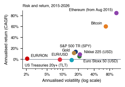


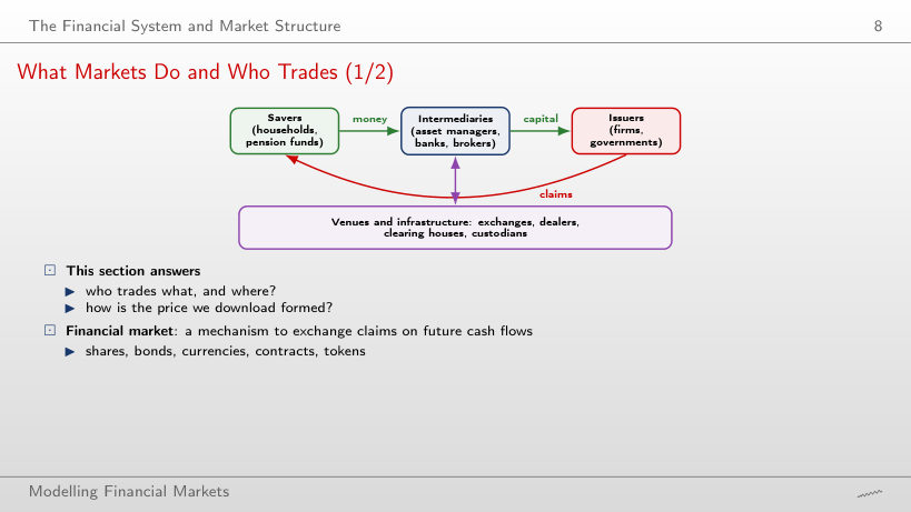
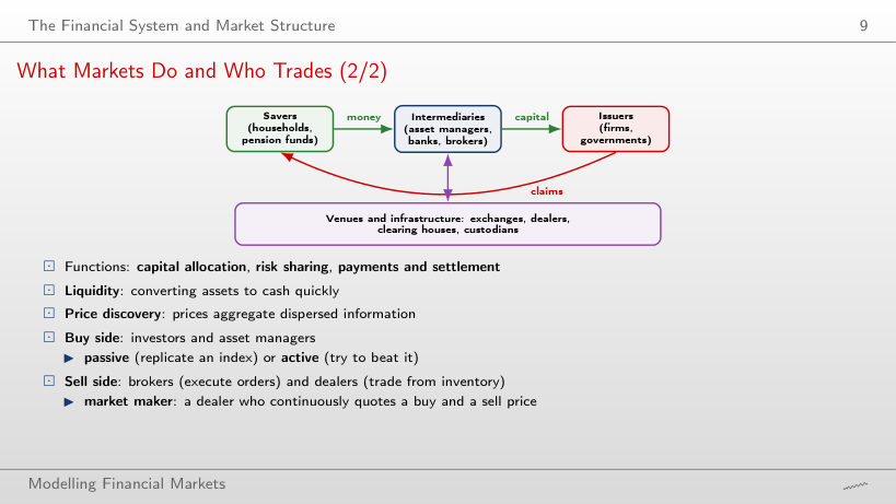
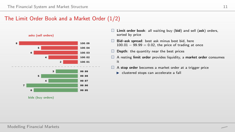
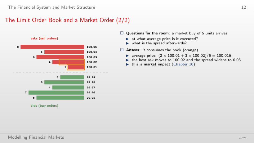
 MFM_ch0_history






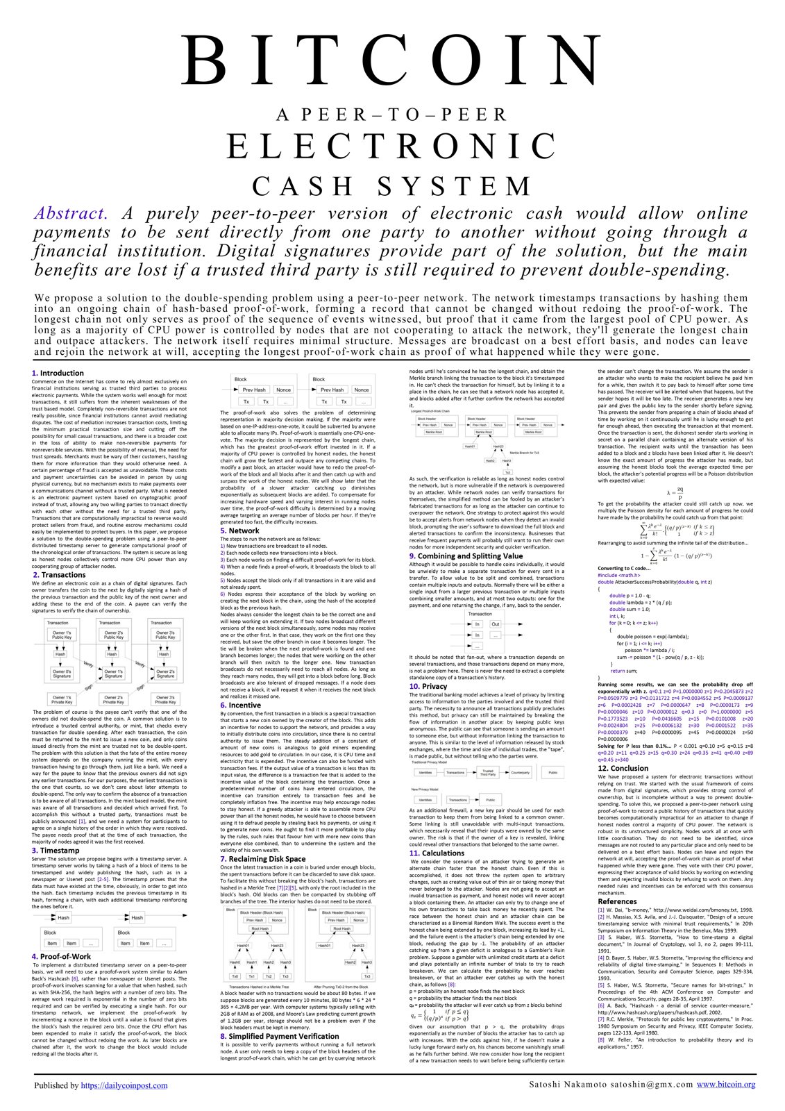
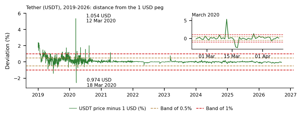
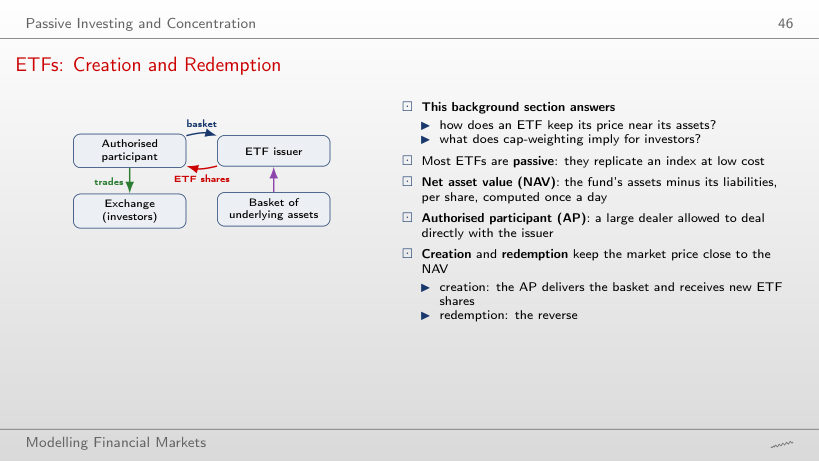

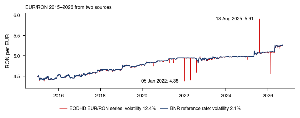
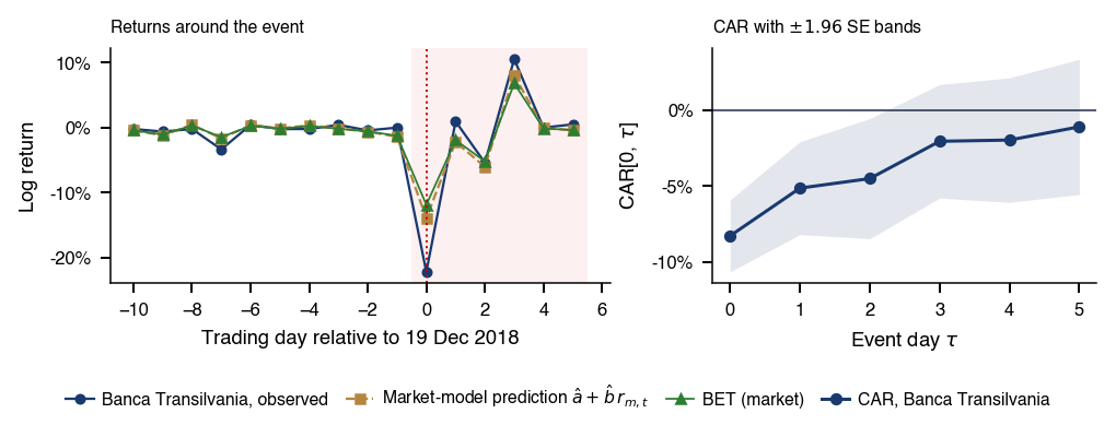
 Statistics of Financial Markets