Bucharest University of Economic Studies IDA Institute Digital Assets Blockchain Research Center AI4EFin Artificial Intelligence for Energy Finance Romanian Academy, Institute for Economic Forecasting MSCA Digital Finance
“This paper presents a method for inferring the effective bid-ask spread directly from a time series of market prices. The method requires no data other than the prices themselves; so it is very cheap.” — Roll (1984)
One tick (USD 0.01) on SPY (SPDR S&P 500 ETF Trust, an exchange-traded fund on the S&P 500) is 0.21 bp: the floor of the quoted spread
From daily bars, the SPY spread estimates lie two orders of magnitude above one tick
Roll 64.3 bp, EDGE (Efficient Discrete Generalized Estimator of the spread) 40.1 bp: they are dominated by volatility
From 5-minute bars, EDGE gives 0.46 bp, the closest to one tick
Corwin–Schultz puts the BVB (median 54 bp) next to the US (median 53 bp)
median daily traded value: USD 0.34 million on the BVB, USD 10 505 million in the US
This paper presents a method for inferring the effective bid-ask spread directly from a time series of market prices. The method requires no data other than the prices themselves; so it is very cheap.
The chapter asks two questions: what does trading cost, and how do prices incorporate information, when orders are matched by computers in microseconds? The most direct cost is the effective spread, measured from trades and quotes. Roll (1984) showed that in an efficient market the spread can be inferred from prices alone, from the autocovariance of price changes. The Corwin–Schultz, Abdi–Ranaldo and EDGE (Efficient Discrete Generalized Estimator, of the bid-ask spread) estimators build on the same idea of inferring the cost from prices alone.
For SPY, a tick of USD (US dollar) 0.01 is 0.21 bp. It is a floor for the quoted spread, not for the effective one. From daily bars, September 2024 to September 2026, the estimates lie two orders of magnitude above a tick: Roll 64.3 bp, Corwin–Schultz 26.5 bp, Abdi–Ranaldo 55.1 bp and EDGE 40.1 bp. From 5-minute bars, over 1,477 days in 2020–2026, EDGE gives 0.46 bp, with interval [0.41, 0.51] bp, the closest to one tick. The daily estimators are dominated by volatility, not by the cost of trading.
The same problem appears across markets. For 25 assets from the US, the Bucharest Stock Exchange (BVB) and crypto, the median Corwin–Schultz estimate is 53 bp in the US and 54 bp on the BVB, although the median daily traded value is USD 10,505 million in the US and USD 0.34 million on the BVB. The Amihud illiquidity ratio separates the two markets: for Banca Transilvania, the most liquid BVB stock, it is 28.0 bp per USD 1 million, about 17,600 times the value for SPY. The chapter therefore builds the liquidity measures from the limit order book to the Glosten–Milgrom and Kyle models, which explain the spread and price impact through information, and to the optimal execution of a large order.
Bid-ask spread estimates for SPY, in basis points (bp) on a log scale: from daily bars (September 2024 – September 2026) and from 5-minute bars (1,477 days, 2020–2026), compared with a tick of USD 0.01 (0.21 bp). Interactive chart: “Spread Estimators at Two Frequencies: SPY” →
What you will be able to do
Compute the Roll, Corwin–Schultz, Abdi–Ranaldo and EDGE spread estimates.
Compute the Amihud ratio and interpret its units.
Derive the Glosten–Milgrom spread, the Kyle equilibrium and the Almgren–Chriss trajectory.
Interpret information shares and the latency arbitrage tax.
The Limit Order BookLiquidity, orders, priority and matching, a simulated book and the cost of a market order that walks the book.
The Bid-Ask SpreadThe Roll model and the price-based estimators, at two frequencies for SPY and for 25 assets.
Illiquidity and Intraday PatternsThe Amihud ratio across markets and over time, the U shape of the trading day and the link with the VIX (CBOE Volatility IndeX).
Information and PricesThe Glosten–Milgrom and Kyle models, PIN, the empirical lambda and order-flow imbalance (OFI).
Every trade on a modern exchange is the result of an algorithm, the matching engine, that pairs buy and sell orders according to fixed rules. The chapter studies what these rules imply for two quantities: the cost an investor pays to trade, and the speed at which private and public information reaches the price. Both are measured on the course data, which combine 5-minute bars for SPY, the exchange-traded fund (ETF) on the S&P 500 (Standard & Poor's) index, daily bars for US stocks, Bucharest Stock Exchange (BVB) blue chips and crypto-assets, and simulated order books where a mechanism must be seen in isolation.
What We Will Explain: from Orders to Prices and Costs
When computers match orders in microseconds, two questions organise the field of market microstructure: what it costs to trade, and how prices absorb information. The answers depend on the rules of the matching engine itself. Price-time priority, the tick size and the opening and closing auctions all shape the prices observed and the costs paid (Gould et al., 2013). A price series is therefore not a sample from an abstract continuous process but the record of a trading mechanism.
The chapter builds the answers in layers. It starts with the limit order book and with the bid-ask spread, measured either from trades and quotes or, when only prices are available, with the estimators of Roll, Corwin–Schultz, Abdi–Ranaldo and EDGE. It continues with the Amihud illiquidity ratio, which measures price impact from daily data, and with two models in which the spread and price impact arise from private information, those of Glosten–Milgrom and Kyle. The Almgren–Chriss model then turns impact into a schedule for executing a large order.
The applications cover stress episodes, crypto venues, the BVB, the speed race between high-frequency traders and intraday momentum. The worked exercises are in Seminar 10. Detailed examples and advanced topics are in Further Topics, before the Appendix; the reference textbook is Franke, Härdle & Hafner (2019).
Most equity, futures and crypto markets are organised as a continuous limit order book. This section defines liquidity and the elements of the book, states the rules by which orders are matched, and uses a simulated book to show why the cost of a market order rises less than proportionally with its size.
Liquidity is the ability to trade a quantity quickly at a price close to fair value. No single number captures it. Kyle (1985) distinguishes three dimensions:
tightness, the cost of a small round trip, measured by the spread;
depth, the size needed to move the price by a given amount;
resiliency, the speed with which prices recover after a shock.
Harris (2003) adds immediacy, the speed at which an order can be executed. A market can be tight but shallow, or deep but slow to recover, and the measures of this chapter capture different dimensions.
The limit order book (LOB) holds all standing limit orders, ordered by price and by time of arrival (Gould et al., 2013). At time \(t\) its state is summarised by the best bid \(b_t\), the highest price at which someone is willing to buy, and the best ask \(a_t\), the lowest price at which someone is willing to sell, with \(b_t < a_t\). The mid-price and the relative quoted spread are
with the relative spread usually expressed in basis points (1 bp = 0.01%). The depth is the quantity waiting at a price level. The tick size is the smallest permitted price step, USD 0.01 for most US stocks priced above USD 1, so the quoted spread can never be smaller than one tick.
In brief
Question: what does a market order buy, and why does its cost depend on the shape of the book?
Liquidity: trading a quantity quickly at a price close to fair value
no single number captures it
Tightness (the spread), depth (size needed to move the price), resiliency (speed of recovery) Kyle (1985); immediacyHarris (2003)
Limit order book (LOB): all standing limit orders, by price and time of arrival Gould et al. (2013)
At time \(t\): best bid \(b_t\) < best ask \(a_t\)
mid-price \(m_t = (a_t + b_t)/2\)
relative spread \((a_t - b_t)/m_t\) in basis points (1 bp = 0.01%)
Depth: quantity waiting at a price level; tick size: smallest price step (USD 0.01 for most US stocks above USD 1)
A market order is executed immediately against the liquidity available in the book; its execution is certain but its price is not. A limit order fixes the worst acceptable price; its price is bounded but its execution is uncertain. Other order types are described in the Appendix. Resting limit orders supply liquidity, whereas market orders, and limit orders priced to execute at once (marketable limit orders), consume it.
During continuous trading, orders are matched by price-time priority: the better price is served first and, among orders at the same price, the earlier one. Orders at one price therefore form a queue, and a position near its head has value; the case study on the high-frequency trading arms race measures how much the race for it costs. At the open and the close, call auctions pool the orders instead and execute them at the single price that maximises the executed quantity.
A market buy of size \(Q\) larger than the depth at the best ask walks up the book. It is filled at the best ask until that level is exhausted, then at the next level, and so on. Relative to the mid-price it pays the half-spread on the first units and the distance to the deeper levels on the rest.
In brief
Market order: immediate execution against the available liquidity, uncertain price
limit order: price bounded by the limit, uncertain execution
Question for the room Why does the arrival rate of limit orders alone not determine the average depth at a price level?
Answer
Depth is a stock of resting orders; arrivals are a flow. Executions and cancellations determine how long orders remain in the book, and market orders consume the best quotes first. In the simulation, the average depth is 0.8 orders at 1 tick from the mid, 4.8 at 10 ticks and 5.0 at 25 ticks; the spread averages 3.23 ticks.
The chart shows a book generated by a zero-intelligence model of order flow (Farmer, Patelli & Zovko, 2005), in which limit orders, market orders and cancellations arrive at random with fixed rates. The model has no traders with strategies or information; whatever structure the book shows comes only from the arrival process and the matching rules. The left panel is a single snapshot of the book, with bids in green and asks in red; the right panel shows the mean depth as a function of the distance from the mid-price, in ticks.
The rates of the simulation are listed in the Appendix. Over 199 snapshots the mean spread is 3.23 ticks and the median 3 ticks, and the spread exceeds 6 ticks 10% of the time. The mean depth is 0.8 orders at 1 tick from the mid, 4.8 orders at 10 ticks and 5.0 orders at 25 ticks.
The profile of depth is the main lesson of the simulation. Market orders execute against the best levels first, so liquidity close to the price is consumed continuously and remains scarce, while levels far from the price accumulate orders (Tóth et al., 2011). Real order books show the same rise of depth away from the mid (Bouchaud, Bonart, Donier & Gould, 2018). This shape is what makes the cost of a large market order concave in its size, as the next frame shows.
The experiment sends market buys of 1 to 80 units against each simulated snapshot and records two prices: the marginal price, reached by the last unit filled, and the average execution price. Both are measured in ticks above the mid-price and plotted on log-log axes, so that a power law appears as a straight line whose slope is the exponent.
Question for the room Approximate the average cost per unit relative to the mid-price by Q0.44. By what factor does the total cost relative to the mid rise when the order size doubles?
Answer
About 2.71. Total cost is quantity times average cost per unit: 21+0.44 ≈ 2.71. The factor 1.36 = 20.44 applies only to the cost per unit; the factor 2 assumes that it stays constant. The slope 0.44 is fitted over the 10 sizes (the 80-unit order pays 11.9 ticks per unit on average), so the relation is an approximation, not an identity for every pair of orders. The deepest level reached has slope 0.53, close to 1/2: the impact is concave.
A 1-unit order reaches 1.7 ticks above the mid and an 80-unit order 20.1 ticks. The slope of the marginal price is 0.53, close to 1/2: the impact is concave. The average execution price has slope 0.44, and an order of 80 units pays on average 11.9 ticks per unit. Doubling the order therefore multiplies the cost per unit by \(2^{0.44} \approx 1.36\), not by 2, and the total cost, size times cost per unit, by \(2^{1 + 0.44} \approx 2.7\).
The impact is concave because the depth of the book grows with the distance from the mid. Large orders that are split and executed over time, called metaorders, follow a similar law; the section on price impact and optimal execution returns to it.
In brief
Market buys of 1 to 80 units sent against each simulated snapshot; log-log axes
Marginal price: a 1-unit order reaches 1.7 ticks above the mid, an 80-unit order 20.1 ticks
Concave impact: slope 0.53, close to 1/2
Average execution price: slope 0.44; 80 units pay 11.9 ticks per unit on average
Doubling the order: cost per unit \(\times 2^{0.44} \approx 1.36\), not 2
total cost (size \(\times\) cost per unit) \(\times 2^{1 + 0.44} \approx 2.7\)
The impact is concave because book depth grows with distance from the mid
Large orders split over time (metaorders) show a similar law
The limit order book is a queue of standing orders ranked by price and time. The spread measures tightness, and the depth profile determines how far a market order of a given size moves the price; in the simulated book the marginal impact grows roughly as the square root of the size. The next section asks what the spread compensates and how it can be measured when only prices are observed.
The Bid-Ask Spread
The spread is the most direct cost of trading. This section explains which costs it pays for, defines the quoted, effective and realised spreads measured from trades and quotes, and then derives the estimators that infer the spread from prices alone: the Roll covariance estimator and the range-based estimators of Corwin–Schultz, Abdi–Ranaldo and EDGE. The estimators are applied to SPY at two frequencies and to 25 assets from three markets.
A liquidity provider buys at the bid and sells at the ask, and the spread is the payment for this service. Huang & Stoll (1997) decompose it into three costs:
Order processing covers fees, technology and clearing.
Inventory cost compensates the provider for holding an unwanted position, which exposes it to price risk until the position is unwound.
Adverse selection arises because some counterparties know more about the value of the asset than the provider (Bagehot, 1971).
The third component does not disappear with technology or competition. A provider who trades with an informed trader loses on average, because the price moves against the provider after the trade. In a competitive market these losses must be recovered from the uninformed, or noise, traders through the spread. The section Information and Prices derives the size of this component in two models.
In brief
Question: why is there a spread, and how do we measure it with and without quotes?
A liquidity provider buys at the bid and sells at the ask
Three measures describe the cost of a round trip, all expressed relative to the mid-price \(m_t\) prevailing just before the trade. Let \(p_t\) be the trade price and \(q_t\) the trade direction: \(q_t = +1\) if the buyer initiated the trade, by hitting the ask, and \(q_t = -1\) if the seller did. The quoted spread \(S^Q_t\) of (10.1) uses only quotes. The effective and realised spreads are
The effective spread measures what the trade actually paid. The factor \(q_t\) makes the cost positive for buys and sells alike, and the one-way cost is \(S^E_t/2\).
The realised spread replaces the pre-trade mid by the mid \(m_{t+\Delta}\) observed a time \(\Delta\) after the trade, for example 5 minutes. It measures what the liquidity provider keeps, before fees and inventory costs, once the price has moved. It is negative when \(q_t(m_{t+\Delta} - p_t) > 0\), that is, when the later mid-price passes the trade price in the direction of the trade; a smaller continuation lowers \(S^R_t\) but can leave it positive.
In brief
Three measures of what a round trip costs, all relative to the mid-price \(m_t\) just before the trade
\(p_t\): trade price
\(q_t = +1\) if the buyer initiated the trade (it hit the ask), \(-1\) if the seller did
The difference between the two measures in (10.2) is the price impact, \(S^E_t - S^R_t = 2 q_t (m_{t+\Delta} - m_t)/m_t\), the lasting move of the mid-price in the direction of the trade. It is usually attributed to adverse selection, because a lasting move indicates that the trade carried information; inventory effects and order-flow pressure also contribute.
Effective and realised spreads require trades, the quotes prevailing at each trade and the direction of each trade. Public data rarely record the direction, so it is inferred, for example by the rule of Lee & Ready (1991): a trade above the mid-price is classified as a buy, a trade below it as a sell, and a trade at the mid by the tick test, which compares its price with the last different trade price. When such data are not available, the spread can only be estimated from prices, the subject of the next frames.
In brief
Price impact: \(S^E_t - S^R_t = 2 q_t (m_{t+\Delta} - m_t)/m_t\), the lasting move of the mid
usually attributed to adverse selection
inventory and order-flow pressure also contribute
Effective and realised spreads need trades, the prevailing quotes and the trade direction
Roll (1984) observed that the spread leaves a trace in the time series of trade prices, which bounce between the bid and the ask. Consider successive trades \(t = 1, \dots, n\), with prices in USD or in logs. The efficient price is a random walk that moves only on news, \(m_t = m_{t-1} + \varepsilon_t\), with \(\varepsilon_t\) independent and identically distributed (i.i.d.), with mean 0 and variance \(\sigma^2\). The trade price is \(p_t = m_t + c\,q_t\), where \(c > 0\) is the half-spread, so the spread is \(s = 2c\), and the sign \(q_t\) is \(+1\) (a buy at the ask) or \(-1\) (a sell at the bid) with probability 1/2, i.i.d. and independent of \(\varepsilon\).
The price change is \(\Delta p_t = \varepsilon_t + c(q_t - q_{t-1})\). Its variance and first-order autocovariance are
The negative autocovariance is the bid-ask bounce. The sign \(q_{t-1}\) enters \(\Delta p_{t-1}\) with coefficient \(+c\) and \(\Delta p_t\) with coefficient \(-c\), so a move up to the ask tends to be followed by a fall back to the bid, even though the efficient price is a random walk. Inverting (10.3) gives the Roll estimator
\[\hat s = 2\hat c = 2\sqrt{-\widehat{\operatorname{Cov}}(\Delta p_t, \Delta p_{t-1})},\]
(10.4)
where \(\widehat{\operatorname{Cov}}\) is the sample first-order autocovariance of the \(n - 1\) price changes. The estimator is defined only when this autocovariance is negative.
In brief
Idea Roll (1984): the spread can be read from the way trade prices bounce between bid and ask
Bid-ask bounce: the common term \(q_{t-1}\) enters \(\Delta p_{t-1}\) with \(+c\) and \(\Delta p_t\) with \(-c\), so a jump up to the ask tends to be followed by a fall to the bid, even when the efficient price is a random walk
Roll estimator: \(\hat s = 2\hat c = 2\sqrt{-\widehat{\Cov}(\Delta p_t, \Delta p_{t-1})}\)
\(\widehat{\Cov}\): the sample first-order autocovariance of the \(n - 1\) price changes
The simulation generates \(n = 5{,}000\) trades from the Roll model with half-spread \(c = 0.05\) and news volatility \(\sigma = 0.02\), so the true spread is \(2c = 0.10\). The left panel shows the first 80 trades, with the efficient price \(m_t\) and the trade price \(p_t\). The right panel shows the autocorrelations of the price changes of both series up to lag 8. The light-blue band, \(\pm 1.96/\sqrt{n}\), is the pointwise 95% band for the autocorrelations of white noise, and the dashed line marks the theoretical first-order autocorrelation.
Question for the room Keep σ = 0.02 and double the half-spread c from 0.05 to 0.10. What is the theoretical first-order autocorrelation of trade-price changes?
Answer
About −0.490: ρ1 = −c²/(σ² + 2c²) = −0.01/0.0204. The autocorrelation does not double, because c also enters the denominator. At c = 0.05 the estimate is −0.458, against −0.463 theoretically, and the Roll estimator gives ŝ = 0.0998, against the true spread 2c = 0.10. Beyond lag 1 the autocorrelations are small, but the one at lag 3 (0.0278) lies very slightly outside the 95% band (0.0277): the band is pointwise and does not cover all lags simultaneously.
The Roll estimate is \(\hat s = 0.0998\), against the true 0.10. The lag-1 autocorrelation of trade-price changes is \(-0.458\), against the theoretical value \(-c^2/(\sigma^2 + 2c^2) = -0.463\) implied by (10.3). At lags 2 to 8 the autocorrelations of trade prices lie inside the pointwise 95% band; the lag-3 value, 0.028, sits right at its edge.
The absence of significant autocorrelation beyond lag 1 is compatible with weak-form efficiency at these lags, but it does not prove it. Trade prices are still not a random walk: the first lag carries the bounce.
In brief
Left: the first 80 trades, efficient price \(m_t\) and trade price \(p_t\)
right: autocorrelations of the price changes up to lag 8, for both prices
On real data the sample autocovariance is often positive, and then the Roll estimate does not exist. On SPY 5-minute bars this happens on 41% of days. Two explanations compete:
Under sampling error the model is true, but the number of observations is small and \(c^2\) is small relative to \(\sigma^2\), so the estimate is dominated by noise.
Under misspecification the model is wrong: prices trend after news, orders are split into many trades, prices are stale, or bars are used instead of individual trades.
The notation of Harris (1990) makes the sampling problem precise. Let \(\gamma_k = \operatorname{Cov}(\Delta p_t, \Delta p_{t-k})\), so that \(\gamma_0 = \sigma^2 + 2c^2\) and \(\gamma_1 = -c^2\) in the Roll model. Let \(T\) be the number of price changes, 77 per day for SPY, and \(\hat\gamma_1\) the sample autocovariance computed from demeaned price changes. The estimate is biased and noisy:
The bias is negative even with no spread (\(c = 0\)), so the Roll estimator then finds a spread that is not there. The variance limit holds for independent signs \(q_t = \pm 1\), and the variance shrinks only as \(1/T\). Bartlett's Gaussian approximation, \(\gamma_0^2 + 3\gamma_1^2\), omits the fourth cumulant of binary signs, \(-2c^4 = -2\gamma_1^2\). The limit also requires a finite fourth moment, which Chapter 1 questions.
Because \(\hat\gamma_1\) is approximately Normal, the probability of the wrong sign is \(P(\hat\gamma_1 > 0) \approx \Phi(\sqrt{T}\,\gamma_1/\gamma_0)\), where \(\Phi\) is the distribution function of the standard Normal distribution. This probability is close to 1/2 whenever \(c^2 \ll \sigma^2/\sqrt{T}\).Further Topics add the demeaning shift to this formula and compare it with the SPY data.
In brief
On real data the sample covariance is often positive, so \(\hat s\) does not exist
on SPY 5-minute bars, on 41% of days
Sampling error: the model is true, but the sample is short and \(c^2\) is small relative to \(\sigma^2\)
Misspecification: trends after news, orders split into many trades, stale prices, bars instead of trades
\(\gamma_0 = \sigma^2 + 2c^2\) and \(\gamma_1 = -c^2\) in the Roll model
\(T\): the number of price changes (77 per SPY day)
\(\hat\gamma_1\): the sample value, from demeaned price changes
Bias: \(\E[\hat\gamma_1] \approx \gamma_1 - (\gamma_0 + 2\gamma_1)/T\), negative even with no spread (\(c = 0\))
Roll then finds a spread that is not there
Noise: \(T\,\Var(\hat\gamma_1) \to \gamma_0^2 + \gamma_1^2\) as \(T \to \infty\) (independent signs \(q_t = \pm 1\)), so the variance shrinks only as \(1/T\)
Bartlett's Gaussian approximation, \(\gamma_0^2 + 3\gamma_1^2\), omits the fourth cumulant of binary signs: \(-2c^4 = -2\gamma_1^2\)
the limit requires a finite fourth moment, which Chapter 1 questions
Wrong sign: \(\hat\gamma_1\) is approximately Normal, so \(P(\hat\gamma_1 > 0) \approx \Phi(\sqrt{T}\,\gamma_1/\gamma_0)\)
\(\Phi\): distribution function of the standard Normal distribution
close to 1/2 whenever \(c^2 \ll \sigma^2/\sqrt{T}\)
Corwin & Schultz (2012) use the daily high and low instead of the autocovariance. The daily high is usually a buy at the ask and the low a sell at the bid, so the high-low range contains the volatility of the efficient price plus the spread. The two parts scale differently with the length of the interval: the volatility part grows with it, the spread part does not. Comparing one-day and two-day ranges separates them.
Let \(H_t\) and \(L_t\) be the high and low of day \(t\), and \(H_{t,t+1}\),\(L_{t,t+1}\) the high and low over days \(t\) and \(t+1\). Define the sum of the two squared one-day log ranges and the squared two-day log range,
Without a spread, \(\gamma \approx \beta\) on average, because variance adds up over two days; the spread inflates \(\beta\) twice and \(\gamma\) only once. Solving the two moment equations gives
where \(\alpha\) is the spread part of the log range and \(\hat S\) the relative spread, a fraction of the price (multiplied by \(10^4\) for basis points), with \(\hat S \approx \alpha\) for small \(\alpha\).Further Topics show how to read an estimate and check (10.6) on two limit cases.
In brief
Idea Corwin & Schultz (2012): the daily high is usually a buy at the ask, the low a sell at the bid
so the high-low range contains volatility plus the spread
The volatility part grows with the length of the interval, the spread part does not
compare one day with two days
\(H_t\), \(L_t\): high and low of day \(t\)
\(H_{t,t+1}\), \(L_{t,t+1}\): high and low over days \(t\) and \(t+1\)
\(\ln(H/L)\): the log range
\(\beta = \sum_{j=0}^{1}\left[\ln \frac{H_{t+j}}{L_{t+j}}\right]^2\), the sum of the two squared one-day ranges
\(\gamma = \left[\ln \frac{H_{t,t+1}}{L_{t,t+1}}\right]^2\), the squared two-day range
Without a spread, \(\gamma \approx \beta\) on average (variance adds up over two days); the spread inflates \(\beta\) twice, \(\gamma\) only once
Solving the two moment equations: \(\;\alpha = \dfrac{\sqrt{2\beta} - \sqrt{\beta}}{3 - 2\sqrt{2}} - \sqrt{\dfrac{\gamma}{3 - 2\sqrt{2}}}, \qquad \hat S = \dfrac{2(e^{\alpha} - 1)}{1 + e^{\alpha}}\)
\(\alpha\): the spread part of the log range; \(\hat S\): relative spread, a fraction of the price (\(\times 10^4\) for bp), with \(\hat S \approx \alpha\) for small \(\alpha\)
Abdi & Ranaldo (2017) combine the close with the range. The close is a trade, so it sits at the bid or at the ask, and the middle of the day's range is a proxy for the mid-price. Let \(c_t\) be the log closing price of day \(t\) and \(\eta_t = (\ln H_t + \ln L_t)/2\) the log mid-range. The product of the distances of the close from today's and tomorrow's mid-range is, on average, a quarter of the squared spread:
The argument resembles Roll's. News moves \(\eta_{t+1}\) independently of the bounce at \(c_t\), so the volatility terms average out and only the spread term survives. In practice the expectation is replaced by the sample mean over days, and a negative mean product gives \(\hat S = 0\).
EDGE, the Efficient Discrete Generalized Estimator of Ardia, Guidotti & Kroencke (2024), uses all four prices of a bar: open, high, low and close (OHLC). It builds two moment conditions, each a product of log returns between the open, the close and the mid-range \(\eta_t\), whose exact form is given in the Appendix. Each yields an unbiased estimate of \(S^2\),\(\hat e_1\) and \(\hat e_2\), with sampling variances \(v_1\) and \(v_2\). The two estimates are combined with minimum variance under a diagonal weighting:
Each estimate is weighted by the variance of the other, so the noisier one receives the smaller weight.
Abdi–Ranaldo and EDGE share two practical features: they need only OHLC bars, and a negative mean moment gives \(\hat S = 0\). Neither yields an exactly unbiased estimate of \(S\), because \(\sqrt{\hat S^2}\) is a concave transformation of an unbiased estimate of \(S^2\). For crypto-assets, Brauneis, Mestel, Riordan & Theissen (2021) find that high-low estimators track the time variation of liquidity measured at high frequency, while the Amihud ratio is better for levels.
Two moment conditions, each a product of log-returns between the open, the close and \(\eta_t\) (exact form: Appendix), give two unbiased estimates \(\hat e_1\), \(\hat e_2\) of \(S^2\), with sampling variances \(v_1\), \(v_2\)
Question for the room EDGE on 5-minute bars has a mean of 0.46 bp and a 95% bootstrap interval of [0.41, 0.51] bp. One tick is 0.21 bp. Does this establish that the true effective spread exceeds 0.21 bp?
Answer
No. The interval, from a 20-day block bootstrap, concerns the mean of the EDGE estimates after negative estimates are replaced by zero; it does not automatically cover the true effective spread. One tick is a lower bound for the quoted spread, not for the effective spread; proximity to one tick is only a plausibility check. On daily bars all estimates are two orders of magnitude above one tick (Roll 64.3, Corwin–Schultz 26.5, Abdi–Ranaldo 55.1 and EDGE 40.1 bp), because the daily range is dominated by volatility.
The chart compares the four estimators on SPY, computed once from daily bars and once from 5-minute bars. The vertical axis is the spread estimate in basis points on a log scale; dark-blue bars come from daily bars (September 2024 – September 2026), teal bars from 5-minute bars (1,477 days, 2020–2026), and the red dashed line marks one tick.
One tick, USD 0.01, is 0.21 bp of the SPY price. It is a floor for the quoted spread but not for the effective spread, since trades can execute inside the quotes. From daily bars the four estimates lie two orders of magnitude above a tick: Roll 64.3 bp, Corwin–Schultz 26.5 bp, Abdi–Ranaldo 55.1 bp and EDGE 40.1 bp. At this frequency the estimators are dominated by volatility, as Jahan-Parvar & Zikes (2023) show for low-frequency spread estimators.
From 5-minute bars the estimates fall by an order of magnitude: Roll 2.82 bp, Corwin–Schultz 3.11 bp, Abdi–Ranaldo 1.06 bp and EDGE 0.46 bp, the closest to a tick, with an interval of [0.41, 0.51] bp. EDGE is computed for each day from its 5-minute bars, negative days are set to 0, and the daily values are averaged; the interval for the mean of the estimator comes from a percentile bootstrap over overlapping 20-day blocks.
A tick is a plausibility check, not a validation, and the result supports a comparison of procedures rather than a measurement of the SPY spread. The Roll estimate of 2.82 bp illustrates the point: about 54% of the mean autocovariance behind it is the demeaning bias of (10.5), and after the correction the Roll spread falls to 1.92 bp, about 32% lower (Further Topics).
In brief
Chart: each estimator in bp, log scale
dark blue: from daily bars (Sep 2024 – Sep 2026)
teal: from 5-minute bars (1 477 days, 2020–2026)
red dashed line: one tick
One tick (USD 0.01) is 0.21 bp: a floor for the quoted spread, not for the effective one
From daily bars the estimates are two orders of magnitude above a tick, dominated by volatility Jahan-Parvar & Zikes (2023)
Roll 64.3, Corwin–Schultz 26.5, Abdi–Ranaldo 55.1, EDGE 40.1 bp
From 5-minute bars EDGE is the closest to a tick
Roll 2.82, Corwin–Schultz 3.11, Abdi–Ranaldo 1.06, EDGE 0.46 bp (interval [0.41, 0.51])
EDGE per day from its 5-minute bars, negative days set to 0, then averaged
interval for the mean of the estimator: percentile bootstrap over overlapping 20-day blocks
A tick is a plausibility check, not a validation
Type of evidence: comparison of procedures (it shows which method works better on the same data, not why)
Roll 2.82 bp: about 54% of the mean autocovariance is demeaning bias (Further Topics)
after the correction the Roll spread falls to 1.92 bp, about 32% lower
Question for the room The median Corwin–Schultz estimates are 53 bp in the US and 54 bp on the BVB. What can we infer about the effective spreads of the two groups?
Answer
Similar proxy values do not establish similar effective spreads. Estimates from daily bars rank the assets by volatility (the Spearman correlation with annualised volatility is 0.94), which describes the ranking without validating the level of trading costs; that requires an independent benchmark from trades and quotes. The median daily traded value, USD 10,505 million in the US and USD 0.34 million on the BVB (a ratio of about 31,000), warrants caution.
The chart applies two of the daily estimators to 25 assets: US large caps, BVB blue chips and crypto-assets. For each asset the solid bar is the Corwin–Schultz estimate and the hatched bar the Abdi–Ranaldo estimate, in basis points; colours mark the three markets. The data are daily bars from September 2024 to September 2026, with BVB stocks priced in lei.
The median Corwin–Schultz estimate is 53 bp in the US, 54 bp on the BVB and 124 bp for crypto. Taken at face value, BVB blue chips are as liquid as US large caps. The conclusion is implausible given how little the BVB trades: over the same window and for the same groups, the median daily traded value is USD 10,505 million in the US and USD 0.34 million on the BVB, a ratio of about 31,000.
The ranking follows volatility rather than trading costs, consistent with the SPY comparison at two frequencies. The Abdi–Ranaldo estimate is 0 for 8 of the 25 assets, because the sample mean in (10.7) is negative. Levels of trading costs need an independent benchmark, the effective spread measured from trades (Jahan-Parvar & Zikes, 2023). The result supports a description of what the daily proxies do, not a ranking of markets by cost.
In brief
Chart: Corwin–Schultz (solid bar) and Abdi–Ranaldo (hatched bar), in bp, for each asset
colours: US, BVB, crypto
Daily bars, Sep 2024 – Sep 2026; BVB stocks in lei
Median Corwin–Schultz: US 53, BVB 54, crypto 124 bp
BVB blue chips look as liquid as US large caps
implausible, given how little value they trade (next section)
Median daily traded value, same window and groups: USD 10 505 million in the US, USD 0.34 million on the BVB, a ratio of about 31 000
The ranking follows volatility
Abdi–Ranaldo is 0 for 8 of the 25 assets (negative sample mean)
The spread pays for order processing, inventory risk and adverse selection. Measured from trades and quotes, the effective spread splits into a realised part, kept by the liquidity provider, and price impact. Estimated from prices alone, the spread is identified only when the bounce is large relative to volatility: on daily bars all four estimators mostly measure volatility, and on SPY 5-minute bars EDGE comes closest to one tick. The next section turns to price impact, which separates markets that daily spread proxies cannot tell apart.
Illiquidity and Intraday Patterns
Spread estimators measure the cost of a small trade. For most investors the larger cost is price impact, the amount by which trading moves the price. This section measures it with the Amihud ratio, which needs only daily returns and traded values, compares 25 assets and three markets over time, asks whether illiquidity is priced, and then looks inside the trading day of SPY.
where \(r_{i,d}\) is the daily return and \(\mathrm{DVOL}_{i,d}\) the traded value, price times volume. With \(r\) as a fraction and DVOL (Dollar VOLume, traded value, price × volume) in USD, the scale \(K = 10^4 \times 10^6 = 10^{10}\) expresses the ratio in basis points of price move per USD 1 million traded. A larger value means a less liquid asset: the same traded value moves the price more.
The ratio needs only daily returns and volumes, which exist for every market and period. For BVB stocks traded values in lei are converted at the reference rate of the National Bank of Romania (BNR) for the day, and for crypto-assets the traded value in USD is summed across exchanges. The ratio is a low-frequency proxy of Kyle's lambda, the price move per unit of order flow defined in the section Information and Prices(Hasbrouck, 2009).
In brief
Question: how do we measure market depth with only daily returns and volumes?
Daily price impact per unit of money traded Amihud (2002): \(\;\mathrm{ILLIQ}_i = \dfrac{K}{D_i}\displaystyle\sum_{d=1}^{D_i} \dfrac{|r_{i,d}|}{\mathrm{DVOL}_{i,d}}\)
\(i\): the asset; \(d = 1, \dots, D_i\): its trading days with nonzero volume; \(r_{i,d}\): daily return; \(\mathrm{DVOL}_{i,d}\): traded value (price \(\times\) volume)
\(K = 10^4 \times 10^6 = 10^{10}\), with \(r\) as a fraction and DVOL (Dollar VOLume, traded value, price × volume) in USD: basis points of price move per USD 1 million traded
Larger means less liquid: the same traded value moves the price more
Needs only daily returns and volumes, available for every market and period
BVB stocks: lei at the BNR (Banca Națională a României, the National Bank of Romania) reference rate of the day
crypto: traded value in USD summed across exchanges
A low-frequency proxy of Kyle's lambda (section Information and Prices) Hasbrouck (2009)
A toy day fixes the units. A return of 50 bp in absolute value on USD 25 million traded gives \(50/25 = 2\) bp per USD 1 million, or 200 bp per USD 100 million. The ratio in (10.9) averages such daily values over the sample.
The intraday SPY measure used later in this section is expressed in bp per USD 100 million and is the mean of the day's 78 bar ratios. Its sample mean, 1.83, is 0.0183 bp per USD 1 million. It is not comparable with the daily SPY ratio of 0.0016: a 5-minute bar carries about 1/78 of the day's traded value, but its absolute return is not 78 times smaller than the daily one.
The link with Kyle's \(\lambda\), the price move per share of net order flow \(y\), follows from a bound. If all volume were net flow, a move \(\Delta p = \lambda y\) at price \(p\) would give
Offsetting buys and sells add volume without moving the price, so the observed ratio is at most \(\lambda/p^2\); seminar exercise A6 works through the argument.
In brief
A toy day: \(|r| = 50\) bp on USD 25 million traded gives \(50/25 = 2\) bp per USD 1 million
i.e. 200 bp per USD 100 million
\(\mathrm{ILLIQ}_i\) averages such daily ratios
The intraday SPY measure of this section: bp per USD 100 million
the mean of the day's 78 bar ratios
Its mean 1.83 is 0.0183 bp per USD 1 million, not comparable with the daily SPY ratio (0.0016): a bar carries about 1/78 of the day's value, but its \(|r|\) is not 78 times smaller
Link to Kyle's \(\lambda\), the price move per share of net order flow \(y\)
if all volume were net flow, \(\Delta p = \lambda y\)
at price \(p\): \(|r| = \lambda|y|/p\) and \(\mathrm{DVOL} = p|y|\), so \(|r|/\mathrm{DVOL} = \lambda/p^2\)
Offsetting buys and sells add volume without moving the price, so the ratio is at most \(\lambda/p^2\) (seminar A6)
Question for the room How many times larger is the Amihud ratio of Banca Transilvania, the most liquid BVB stock, than that of SPY?
Answer
About 17,600 times: 28.0 bp against 0.0016 bp per USD 1 million traded. Bitcoin has 0.0037 bp, close to SPY, and Transelectrica 1,024.0 bp. The Amihud ratio separates the three markets by orders of magnitude, which the spread estimators from daily bars do not.
The chart shows the Amihud ratio of each of the 25 assets, in basis points per USD 1 million on a log scale, over September 2024 – September 2026. The ratio is the mean over about 500 trading days, or 730 days for crypto-assets, which trade every day; colours mark the US, the BVB and crypto.
The ratio is 0.0016 bp per USD 1 million for SPY, whose median traded value is USD 40,124 million a day, and 0.0037 bp for Bitcoin. For Banca Transilvania, the most liquid BVB stock, it is 28.0 bp, about 17,600 times the value for SPY. Transelectrica reaches 1,024.0 bp and the BET (Bucharest Exchange Trading, index) ETF 212.9 bp.
The assets form three clusters, orders of magnitude apart: US large caps and the top crypto-assets; smaller crypto-assets and GameStop; and the BVB. The daily spread proxies of the previous section do not separate the markets into these clusters, whereas the Amihud ratio does, because it scales with traded value. The ratio remains a proxy, not a cost at which one could actually trade, and the result supports a description.
In brief
Sep 2024 – Sep 2026, log scale; mean over about 500 trading days (730 for crypto)
SPY 0.0016 bp per USD 1 million; Bitcoin 0.0037 bp
SPY median traded value USD 40 124 million a day
Banca Transilvania, the most liquid BVB stock: 28.0 bp, about 17 600 times SPY
Transelectrica 1 024.0 bp; the ETF on the BET (Bucharest Exchange Trading index, the BVB benchmark): 212.9 bp
Three clusters, orders of magnitude apart
US large caps and top crypto
smaller crypto and GameStop
the BVB
Daily spread proxies do not separate markets into these three clusters
Question for the room Does the decline of the BVB Amihud ratio identify the effect of the move to FTSE (Financial Times Stock Exchange, FTSE Russell, index provider) Russell emerging-market status in September 2020?
Answer
No: the observed path alone provides no counterfactual, and the absence of a visible break does not establish a zero effect either. The mean of the monthly BVB medians falls from 435 bp per USD 1 million in 2017 to 169 bp in January–August 2026; in August 2026 the monthly median is 153 bp, about 7,000 times the US median. The largest decline is in crypto: the annual mean falls from 7.6 bp to 0.089 bp.
The chart shows the monthly Amihud ratio, as the median across the assets of each group, without SPY and the BET ETF, on a log scale. In crypto the median falls from 7.6 bp per USD 1 million in 2017 to 0.089 in 2026, and in the US from 0.062 to 0.023. On the BVB it falls from 435 to 169, still about 7,000 times the US median.
The BVB series shows no visible break at the move to emerging-market status by the index provider FTSE Russell in September 2020 (BVB, 2026). Thin trading also affects the ratio itself: Further Topics show the traded value of the BVB blue chips and the model of nonsynchronous trading.
In brief
Monthly Amihud ratio, median across each group (without SPY and the BET ETF), log scale
Crypto: from 7.6 bp per USD 1 million (2017) to 0.089 (2026); US: from 0.062 to 0.023
BVB: from 435 to 169, still about 7 000 times the US median
no visible break at the move to emerging-market status by the index provider FTSE Russell (FTSE: Financial Times Stock Exchange), September 2020 BVB (2026)
Illiquidity can affect expected returns in three ways:
In levels, investors demand a higher return for assets that are costly to trade (Amihud & Mendelson, 1986); expected return increases with the spread, concavely, because investors with long horizons hold the illiquid assets and amortise the cost over a long holding period.
In the time series, expected market illiquidity raises future returns, and an unexpected rise in illiquidity lowers current prices (Amihud, 2002).
The course data show the time-series effect in three markets. Unexpected illiquidity is the residual of a first-order autoregressive model, AR(1), fitted to the market's monthly illiquidity, as in Amihud (2002). The monthly market return is regressed on last month's illiquidity and on this residual, from November 2016 to August 2026. The \(t\)-statistics of the coefficient on the illiquidity shock are \(-4.0\) on the BVB, \(-3.8\) in the US and \(-4.1\) in crypto (seminar exercise C2): returns fall when illiquidity rises unexpectedly. The result supports an association, since the return and the illiquidity shock are measured in the same month.
In brief
Level: investors demand a higher return for assets that are costly to trade Amihud & Mendelson (1986)
Expected return increases with the spread, concavely: long-horizon investors hold the illiquid assets
Time series: expected market illiquidity raises future returns Amihud (2002)
Evidence here: monthly market returns fall when illiquidity rises unexpectedly on the BVB, in the US and in crypto (seminar C2)
Unexpected illiquidity: the residual of an AR(1) (first-order autoregressive) model fitted to the market's monthly illiquidity, as in Amihud (2002); the monthly return is regressed on last month's illiquidity and this residual (Nov 2016 – Aug 2026)
\(t\)-statistics of the illiquidity-shock coefficient: \(-4.0\) (BVB), \(-3.8\) (US), \(-4.1\) (crypto)
Type of evidence: association (the variables move together; this does not prove causation)
the return and the illiquidity shock are measured in the same month
The chart uses the 78 five-minute bars of each full trading day of SPY, 1,477 days from October 2020 to September 2026, with the first bar starting at the opening price. It shows, by time of day, the share of daily volume traded in each bar and the mean absolute 5-minute return.
Question for the room What share of the daily SPY volume trades in the last 30 minutes of the session?
Answer
18.6%, against 12.7% in the first 30 minutes and 0.9% for one 5-minute bar at midday. The mean absolute return is 10.6 bp in the first bar and 5.1 bp at midday, a ratio of 2.06.
Both curves have a U shape. The first bar carries 5.0% of the day's volume and a midday bar 0.9%, against \(1/78 = 1.28\%\) per bar if volume were spread evenly. The last 30 minutes carry 18.6% of the volume, with confidence interval [18.3, 19.0], against \(6/78 = 7.69\%\) if even.
The mean absolute 5-minute return is 10.6 bp in the first bar and 5.1 bp at midday, a ratio of 2.06 with a 95% confidence interval (CI) of [1.98, 2.15], obtained by resampling whole days (seminar exercise B1). The spikes at 10:00 and 14:00 coincide with scheduled macroeconomic data releases.
In brief
78 five-minute bars a day, 1 477 full days (Oct 2020 – Sep 2026)
the first bar starts at the opening price
Volume: first bar 5.0% of the day, a midday bar 0.9%, against \(1/78 = 1.28\%\) per bar if even
last 30 minutes 18.6% [18.3, 19.0] against \(6/78 = 7.69\%\) if even
Mean absolute 5-minute return \(|r|\): 10.6 bp in the first bar, 5.1 bp at midday
Wood, McInish & Ord (1985) documented that returns and volume are highest at the open and the close for stocks of the New York Stock Exchange (NYSE). Several explanations are offered. At the open, overnight news is absorbed and uncertainty is highest, and informed traders act early, before their information spreads. Noise traders who can choose when to trade cluster together, because liquidity attracts liquidity (Admati & Pfleiderer, 1988). At the close, index funds and ETFs trade at the closing price, which is fixed by the closing auction. Bitcoin, which trades around the clock, shows an analogous pattern by hour (Further Topics).
The practical rule is that an execution algorithm should follow the volume curve, trading more when the market trades more, to reduce its impact; the section on optimal execution formalises the trade-off. The result supports a description: the explanations above are not tested here.
The chart compares a daily intraday illiquidity measure for SPY with the VIX, the index of 30-day implied volatility of the S&P 500 computed from option prices. The illiquidity measure is the mean over the day's 78 bars of the absolute return divided by traded value, in bp per USD 100 million (divide by 100 for USD 1 million); the chart shows monthly means.
Question for the room On daily data, the regression of log SPY illiquidity on the log VIX has slope 0.95. Approximately what percentage change in illiquidity is associated with a 10% rise in the VIX?
Answer
A rise of about 9.5%: the elasticity of illiquidity with respect to the VIX is 0.95, and 0.95 × 10% = 9.5%. This is an association, not an identified causal effect. The daily slope has HAC (Heteroskedasticity and Autocorrelation Consistent, standard errors) standard error 0.12; on monthly means the slope is 1.03. The correlation is 0.58 on daily data and 0.69 on monthly means. In April 2025 illiquidity was 3.04 bp per USD 100 million, against a mean of 1.83.
The correlation with the VIX is 0.58 for daily values and 0.69 for monthly means. The elasticity of log illiquidity with respect to log VIX is 0.95, with a standard error of 0.12 that is robust to heteroskedasticity and autocorrelation (HAC); the fitted relation is in seminar exercise B4.
In brief
Daily intraday illiquidity: mean over the 78 bars of \(|r|\) / traded value
bp per USD 100 million (divide by 100 for USD 1 million)
monthly means shown
Correlation with the VIX (CBOE Volatility IndeX): 0.58 daily, 0.69 for monthly means
elasticity of log illiquidity on log VIX 0.95
HAC standard error, robust to heteroskedasticity and autocorrelation: 0.12
In April 2025 the illiquidity measure reached 3.04, against a sample mean of 1.83. Liquidity dries up precisely when investors most need it, so liquidity risk is correlated with market risk, the mechanism behind the liquidity-adjusted asset pricing model of Acharya & Pedersen (2005). The result supports an association only: the illiquidity ratio contains the absolute return, which rises mechanically with volatility.
the illiquidity ratio contains \(|r|\), which rises with volatility
Section summary
The Amihud ratio separates the US, crypto and the BVB by orders of magnitude, where spread proxies do not. Illiquidity has fallen over time in all three markets, shocks to it coincide with lower returns, and within the day SPY trades most at the open and the close. Illiquidity also co-moves with the VIX, partly by construction. The next section explains spreads and price impact through private information.
Information and Prices
The adverse-selection component of the spread and the price impact of order flow have a common origin: some traders know more than the market maker. This section derives them in two models, the sequential-trade model of Glosten and Milgrom and the batch-auction model of Kyle, then reviews the empirical measures that follow from the models and the data each needs.
In the model of Glosten & Milgrom (1985) the asset has value \(V \in \{V_L, V_H\}\), with \(P(V = V_H) = \theta\). In each period one trader arrives. With probability \(\mu\) the trader is informed and buys if \(V = V_H\) and sells if \(V = V_L\); otherwise the trader is a noise trader, uninformed and trading for liquidity needs, who buys or sells with probability 1/2 (Bagehot, 1971). A competitive, risk-neutral market maker earns zero expected profit on each trade, so the ask and the bid are conditional expectations:
A buy signals a high value and a sell a low one, so \(a > b\). The conditional probabilities of a buy follow from the composition of traders: informed traders always buy when \(V = V_H\) and noise traders half of the time, so \(P(\text{buy} \mid V_H) = \mu + \tfrac{1-\mu}{2}\) and \(P(\text{buy} \mid V_L) = \tfrac{1-\mu}{2}\). After each trade the market maker updates \(\theta\) by Bayes' rule: a buy raises it and a sell lowers it.
In brief
Question: how does private information enter prices, and why does it alone create a spread?
Value \(V \in \{V_L, V_H\}\), \(P(V = V_H) = \theta\); each period one trader arrives Glosten & Milgrom (1985)
With probability \(\mu\) informed (buys if \(V = V_H\), sells if \(V = V_L\)), otherwise a noise trader, uninformed and trading for liquidity needs (buys or sells with probability 1/2) Bagehot (1971)
Competitive, risk-neutral market maker with zero expected profit on each trade
The numerator is the probability of a high value and a buy, and the denominator the total probability of a buy. The bid follows symmetrically from a sell. At \(\theta = 1/2\) the spread is \(a - b = \mu(V_H - V_L)\), linear in the share of informed traders: with \(V_L = 90\) and \(V_H = 110\) it is 2 for \(\mu = 0.1\) and 6 for \(\mu = 0.3\).
The model has no inventory and no fees, so the spread exists purely because of information. Because each trade price is a conditional expectation of \(V\) given the history of trades, trade prices form a martingale and the market is efficient in the semi-strong sense of Chapter 2. A simulation of the model, with the speed at which prices discover the true value, is in Further Topics.
In brief
Bayes' rule after a buy, then the ask as the expected value
Kyle (1985) replaces the sequence of single trades by a batch auction with a strategic insider. The insider knows the value \(v \sim N(p_0, \sigma_v^2)\), where \(p_0\) is the price before trading, and submits a market order \(x\). Noise traders submit \(u \sim N(0, \sigma_u^2)\), independent of \(v\). The market maker sees only the total order flow \(y = x + u\) and sets the price \(p = \mathbb{E}[v \mid y]\). A linear equilibrium has the form
\[x = \beta (v - p_0), \qquad p = p_0 + \lambda y,\]
(10.12)
where \(\beta > 0\) is the insider's trading intensity and \(\lambda > 0\) is Kyle's lambda, the price move per share of net order flow.
The insider takes the pricing rule as given and maximises the expected profit \(\mathbb{E}[(v - p)\,x \mid v] = (v - p_0)x - \lambda x^2\): the gain from information minus the cost of moving the price against himself. The first-order condition gives \(x = (v - p_0)/(2\lambda)\), so \(\beta = 1/(2\lambda)\); the insider trades less aggressively because his order moves the price. The market maker, for whom \((v, y)\) is jointly Normal, sets \(\lambda = \operatorname{Cov}(v, y)/\operatorname{Var}(y) = \beta\sigma_v^2/(\beta^2\sigma_v^2 + \sigma_u^2)\), the population slope of an ordinary least squares (OLS) regression of \(v\) on \(y\).
In brief
One insider knows \(v \sim N(p_0, \sigma_v^2)\), with \(p_0\) the price before trading, and submits a market order \(x\)Kyle (1985)
Noise traders submit \(u \sim N(0, \sigma_u^2)\), independent of \(v\)
The market maker sees only the total order flow \(y = x + u\) and sets \(p = \E[v \mid y]\)
Linear equilibrium: \(x = \beta (v - p_0)\), \(p = p_0 + \lambda y\)
\(\beta > 0\): the insider's trading intensity (not the Corwin–Schultz \(\beta\))
\(\lambda > 0\): Kyle's lambda, the price move per share of net order flow
The insider takes the pricing rule as given: \(\E[(v - p)\,x \mid v] = (v - p_0)x - \lambda x^2\)
the gain from information minus the cost of moving the price against himself
First-order condition: \(x = (v - p_0)/(2\lambda)\), so \(\beta = 1/(2\lambda)\): he trades less because his order moves the price
The market maker: \((v, y)\) is jointly Normal, so \(\lambda = \Cov(v, y)/\Var(y) = \beta\sigma_v^2/(\beta^2\sigma_v^2 + \sigma_u^2)\)
the population OLS (ordinary least squares) slope of \(v\) on \(y\)
The comparative statics are direct. More noise trading, a larger \(\sigma_u\), lowers \(\lambda\), so the market is deeper, and raises both the insider's intensity and his profit. More valuable information, a larger \(\sigma_v\), raises \(\lambda\): the market maker protects himself by moving the price more per unit of flow.
Two further properties describe what the price reveals. The insider's order has variance \(\operatorname{Var}(x) = \beta^2\sigma_v^2 = \sigma_u^2\), as large as that of noise trading, behind which he hides. The posterior variance is \(\operatorname{Var}(v \mid y) = \sigma_v^2 - \lambda^2\operatorname{Var}(y) = \sigma_v^2/2\): the price reveals half of the private information.
In brief
Substituting \(\beta = 1/(2\lambda)\) into the slope gives \(\beta^2\sigma_v^2 = \sigma_u^2\), hence
Question for the room In the Kyle model, σv halves and σu doubles. What happens to the expected profit of the insider?
Answer
It stays the same. Expected profit is σvσu/2, so the two changes offset each other: from σv = USD 2 and σu = 10 thousand shares to USD 1 and 20 thousand shares, the profit stays at USD 10 thousand. λ = σv/(2σu), by contrast, falls fourfold, from 0.10 to 0.025 USD per thousand shares. The price still reveals half of the private information.
The chart plots the equilibrium (10.13) as a function of the amount of noise trading, for a fixed value uncertainty. The horizontal axis is \(\sigma_u\), in shares; one curve shows Kyle's lambda and the other the insider's expected profit.
The chart uses \(\sigma_v = 2\) USD and noise trading \(\sigma_u\) from 2,000 to 40,000 shares. Lambda is shown in USD per thousand shares; its inverse, \(1/\lambda\), is market depth, the order flow needed to move the price by one unit. Lambda falls like \(1/\sigma_u\) and the insider's profit rises linearly in \(\sigma_u\), as (10.13) states. Noise traders are both the source of depth and the counterparty that pays for the insider's gain.
In brief
\(\sigma_v = 2\) USD; noise trading \(\sigma_u\) from 2 000 to 40 000 shares
Chart units: \(\lambda\) in USD per thousand shares; \(1/\lambda\) is market depth
Reading the chart: \(\lambda\) falls like \(1/\sigma_u\), the insider's profit rises linearly in \(\sigma_u\)
The probability of informed trading (PIN) of Easley, Kiefer, O'Hara & Paperman (1996) summarises a sequential-trade model estimated on daily counts of buys and sells:
where \(\alpha\) is the probability of an information event on a day, \(\mu\) the arrival rate of informed orders, and \(\varepsilon_b\),\(\varepsilon_s\) the arrival rates of uninformed buys and sells. With \(\alpha = 0.5\),\(\mu = 2\) and \(\varepsilon_b = \varepsilon_s = 2\), PIN \(= 1/(1 + 2 + 2) = 0.20\): one fifth of expected trades are informed.
PIN is a model-implied share of expected order flow. It does not identify which particular trade was informed. Its estimation, and the reasons why it is numerically fragile, are in the Appendix, and a volume-based variant, VPIN, is discussed in Further Topics.
In brief
PIN (probability of informed trading), from the Easley, Kiefer, O'Hara & Paperman (1996) model of daily buy and sell counts: \(\mathrm{PIN}=\alpha\mu/(\alpha\mu+\varepsilon_b+\varepsilon_s)\), PIN \(\in [0, 1]\)
\(\alpha\) probability of an information event on a day
\(\mu\) arrival rate of informed orders
\(\varepsilon_b\), \(\varepsilon_s\) arrival rates of uninformed buys and sells
Example: \(\alpha=0.5\), \(\mu=2\), \(\varepsilon_b=\varepsilon_s=2\) give \(\mathrm{PIN}=1/(1+2+2)=0.20\): one fifth of expected trades are informed
PIN describes a model-implied share; it does not identify which particular trade was informed
VPIN (Volume-synchronised Probability of INformed trading), a volume-time version: Further Topics
Each model has an empirical counterpart, and each counterpart requires specific data. Kyle's lambda is the price change per unit of signed order flow, and the Amihud ratio is its daily proxy (Hasbrouck, 2009). The model of Madhavan, Richardson & Roomans (1997) (MRR) splits the spread into a permanent, adverse-selection part and a transitory part, and needs signed trades and quotes. The vector autoregression (VAR) of Hasbrouck (1991) measures the long-run response of quotes to a trade innovation, with the same data. PIN is the expected share of informed trades and needs daily buy and sell counts. Order-flow imbalance explains most short-horizon price changes (Cont, Kukanov & Stoikov, 2014) but needs order-book events.
The public bars used in this chapter do not sign trades, so MRR, the VAR and PIN are not estimated here. Their equations are in the Appendix.
In brief
Measure
What it identifies
Data needed
Kyle \(\lambda\)
price change per unit of signed order flow; the Amihud ratio is its daily proxy Hasbrouck (2009)
The public bars used here do not sign trades, so MRR (Madhavan–Richardson–Roomans, structural model of trading costs), the Hasbrouck VAR (Vector AutoRegression) and PIN are not estimated here
The empirical Kyle lambda is estimated by regressing the change in the mid-price over an interval \(k\), for example 5 minutes, on the net signed flow in that interval (Hasbrouck, 2007):
where \(v_t\) is the size of trade \(t\) and \(q_t\) its sign, assigned by the Lee–Ready rule.
Order-flow imbalance (OFI), introduced by Cont, Kukanov & Stoikov (2014), uses the events of the order book rather than trades. Each event \(n\) changes the best prices \(P^b_n\),\(P^a_n\) or the depths \(d^b_n\),\(d^a_n\) at the best quotes, and contributes
with \(\mathrm{OFI}_k = \sum_{n \in k} e_n\) and \(\mathbf{1}\{\cdot\}\) equal to 1 if the condition holds and 0 otherwise. A rising bid or a rising ask contributes positively, a falling bid or a falling ask negatively, and at an unchanged quote the change in quantity matters: a fall in the depth at the ask contributes positively.
The relation \(\Delta m_k = \beta\,\mathrm{OFI}_k + \varepsilon_k\) is linear, with \(\beta\) inversely proportional to the average depth at the best quotes, unlike the concave impact of trade volume. Because OFI counts limit orders and cancellations, not only trades, it explains short-horizon price changes better than the trade imbalance. It needs order-book events, which the bars used here do not contain.
In brief
Question: how much does order flow move the price over short intervals, measured directly from data?
Empirical Kyle lambda: regress the mid-price change on the net signed flow Hasbrouck (2007)
a rising bid or a rising ask contributes positively; a falling bid or a falling ask contributes negatively
at an unchanged ask the quantity matters: a fall in \(d^a\) contributes positively
\(\Delta m_k = \beta\,\mathrm{OFI}_k + \varepsilon_k\), with the slope \(\beta\) (not Kyle's) inversely proportional to the average depth at the best quotes: a linear relation, unlike the concave impact of trade volume
OFI counts limit orders and cancellations, not only trades
so it explains short-horizon price changes better than the trade imbalance
it needs order-book events, which the bars used here do not contain
Section summary
In the Glosten–Milgrom model the spread is proportional to the share of informed traders; in the Kyle model the price moves by \(\lambda\) per unit of order flow and reveals half of the private information. PIN, MRR, the Hasbrouck VAR, the empirical lambda and OFI bring these ideas to data, but all require signed trades or order-book events. The next section uses price impact to schedule the execution of a large order.
Price Impact and Optimal Execution
A large order is rarely sent to the market at once. This section states the empirical law of the impact of large orders split over time, sets up the trade-off between impact and price risk in the Almgren–Chriss model, solves it, and reviews the benchmarks against which executions are measured.
The signs of market orders are autocorrelated for hundreds of trades (Bouchaud, Gefen, Potters & Wyart, 2004). The reason is that large orders, called metaorders, are split into many small trades executed over hours or days. Propagator and Hawkes models of this persistence are in the Appendix.
\[\Delta P \approx Y\,\sigma_{\text{day}}\sqrt{\frac{Q}{V_{\text{day}}}},\]
(10.16)
where \(\Delta P\) is the relative price move caused by the metaorder, \(Q\) its size, \(V_{\text{day}}\) the daily volume, \(\sigma_{\text{day}}\) the daily volatility and \(Y\) a constant of order 1. The law is concave: trading 1% of daily volume moves the price by about \(0.1\,\sigma\), not \(0.01\,\sigma\). The reason is the one seen in the simulated book: liquidity near the price is scarce and refills slowly.
If the impact builds as \(I(q) = Y\sigma\sqrt{q/V}\) while the order is executed, where \(q\) is the quantity executed so far, the average price paid is \(\tfrac{2}{3}I(Q)\), before spread and fees. Testing (10.16) requires the traders' own order records; public bars allow only an indirect look (Further Topics).
In brief
Question: how far does a large order move the price?
how should it be split over time to pay as little as possible?
\(\Delta P \approx Y\,\sigma_{\text{day}}\sqrt{Q/V_{\text{day}}}\), with \(\Delta P\) the relative price move caused by the metaorder, \(Q\) its size, \(V_{\text{day}}\) the daily volume, \(\sigma_{\text{day}}\) the daily volatility, \(Y\) a constant of order 1
Concave: trading 1% of daily volume moves the price by about \(0.1\,\sigma\), not \(0.01\,\sigma\)
liquidity near the price is scarce and refills slowly (section The Limit Order Book)
Cost: if impact builds as \(I(q) = Y\sigma\sqrt{q/V}\) during execution, the average price paid is \(\tfrac{2}{3}I(Q)\)
\(q\): quantity executed so far
before spread and fees
Testing it needs the traders' own order records
public bars allow only an indirect look (Further Topics)
Almgren & Chriss (2001) consider an investor who must sell \(X\) shares within \(T\) days, in \(N\) steps of length \(\tau = T/N\). Holdings go from \(x_0 = X\) to \(x_N = 0\), and the trade in step \(k\) is \(n_k = x_{k-1} - x_k\). The market price moves with news and is pushed down by the investor's own sales, while the price received includes a temporary discount:
Here \(\sigma\) is the price volatility in USD per day\(^{1/2}\),\(\xi_k\) an i.i.d. news shock with mean 0 and variance 1, \(\gamma \ge 0\) the permanent impact, which lowers all later prices, and \(\eta > 0\) the temporary impact, paid only by the trade itself.
Trading fast incurs a high temporary impact but little price risk; trading slowly does the opposite. The implementation cost is \(C = X S_0 - \sum_k n_k \tilde S_k\), the value of the position at the initial price \(S_0\) minus what the sales bring. Over deterministic schedules the investor solves
The term \(\eta\,\dot x^2\) makes selling fast costly, and \(\lambda\sigma^2 x^2\) makes holding a large position risky. The solution, derived in the Appendix and in seminar exercise A7, is
The parameter \(\kappa\) measures the urgency of the liquidation: it rises with risk aversion and volatility and falls with the temporary impact, and \(1/\kappa\) is the time scale of the liquidation. With \(\lambda = 0\),\(\kappa = 0\) and holdings fall linearly, so the order is traded evenly. With a large \(\lambda\) most of the order is traded at the start, which cuts the exposure to price risk.
\(\kappa\): the urgency of the liquidation, it rises with risk aversion and volatility, falls with impact; \(1/\kappa\): the time scale of the liquidation
\(\lambda = 0\): \(\kappa = 0\) and holdings fall linearly (trade evenly)
Large \(\lambda\): most of the order is traded at the start, cutting the exposure to price risk
Question for the room If σ doubles, how must λ change to keep the same optimal Almgren–Chriss trajectory, holding the other parameters fixed?
Answer
Divide λ by 4. The trajectory depends on the product λσ², and doubling σ multiplies σ² by 4; this also holds for the discrete formula, in five daily steps, used by the page. Selling 1 million shares over 5 days with λ = 2·10⁻⁶, the standard deviation of the cost falls from USD 1.04 million (selling evenly) to USD 0.45 million, and the expected cost rises from 0.60 to 1.08 million USD; 57% of the position is sold on the first day.
The chart applies (10.19) to the numerical example of Almgren & Chriss (2001). The left panel shows the shares still to sell over the 5 days, for four values of the risk aversion \(\lambda\). The right panel shows the efficient frontier of execution: the expected cost against the standard deviation of cost, both in USD million.
The example sells \(X = 10^6\) shares at \(S_0 = 50\) USD over \(T = 5\) days, with \(\sigma = 0.95\) USD per day\(^{1/2}\),\(\eta = 2.5 \cdot 10^{-6}\) and \(\gamma = 2.5 \cdot 10^{-7}\). With \(\lambda = 2 \cdot 10^{-6}\) the first day sells 57% of the position. The standard deviation of cost falls from 1.04 million USD under even selling to 0.45 million USD, for 0.48 million USD more expected cost.
The frontier is convex: the first units of risk reduction are cheap, the last ones expensive. An investor chooses a point on it according to risk aversion, just as a portfolio is chosen on the mean–variance frontier. The full table is in the Appendix.
In brief
Left: shares still to sell over the 5 days, for four values of \(\lambda\)
right: expected cost against the standard deviation of cost, USD million (the efficient frontier)
Numerical example of Almgren & Chriss (2001): \(X = 10^6\) shares, \(S_0 = 50\) USD, \(T = 5\) days
An execution is judged against a benchmark. The implementation shortfall of Perold (1988) is the difference between a paper portfolio valued at the decision price and the portfolio actually executed; the implementation cost \(C\) of the Almgren–Chriss model is a shortfall of this kind. The volume-weighted average price (VWAP) over the period rewards executions that follow the volume curve, and the time-weighted average price (TWAP) is matched by the even schedule obtained with \(\lambda = 0\).
A participation rule, which trades a fixed share of market volume, ignores price altogether. Such a rule was at the heart of the Flash Crash of 6 May 2010, discussed in the next section.
In brief
Implementation shortfall: paper portfolio at the decision price minus the executed portfolio Perold (1988)
VWAP: the volume-weighted average price over the period
TWAP: the time-weighted one, matched by the \(\lambda = 0\) schedule
A participation rule (a fixed share of market volume) ignores price
the rule at the heart of the Flash Crash (next section)
Section summary
The impact of a metaorder grows with the square root of its size relative to daily volume. The Almgren–Chriss schedule trades impact against price risk: the urgency \(\kappa\) fixes how fast the position is sold, and the efficient frontier of execution prices the reduction in risk. The next section turns to the traders who supply most liquidity today and to what happens when they withdraw it.
High-Frequency Trading and Market Stress
Much of the liquidity in modern equity markets is supplied by algorithms that trade at the scale of microseconds. This section describes what speed changes in liquidity provision, reviews the empirical evidence and models, and documents the Flash Crash of 6 May 2010, when this liquidity disappeared within minutes.
High-frequency trading (HFT) refers to algorithms that trade in micro- to milliseconds and end the day with no open position. Their speed comes from co-location, servers placed next to the exchange's matching engine, and from microwave links that carry signals between trading centres faster than fibre, such as those between Chicago and New Jersey.
Speed changes liquidity provision in two directions:
Low latency speeds up price discovery and narrows spreads (Hasbrouck & Saar, 2013): quotes are updated as soon as prices move elsewhere, so liquidity providers face less risk of being picked off and can quote tighter.
The same liquidity, however, is plentiful in calm markets and fragile under stress, because a fast provider can also withdraw its quotes faster than anyone else.
Menkveld (2013) studies one HFT market maker active on Chi-X and Euronext. Its orders were mostly passive: it earned the spread and lost on its positions, the profile of a classical market maker operating at a much higher frequency. O'Hara (2015) argues that in such markets order flow and latency become sources of information in their own right, alongside fundamental news. Jovanovic & Menkveld (2010) and Pele (2025) model HFT market makers as intermediaries between slower traders.
Inventory shapes how these intermediaries quote. In the model of Avellaneda & Stoikov (2008), a dealer who is long lowers both quotes in order to sell; the model is presented in the Appendix.
Question for the room On 6 May 2010, the SPY low is USD 105.00 and the close USD 112.942. How far is the close above the low, as a percentage of the low?
Answer
About 7.56%: 112.942/105 − 1. The low was 10.1% below the previous close (USD 116.82), and the close 3.3% below it. Volume was 3.0 times the median of the preceding days. Daily bars support these comparisons without describing the fall and the recovery within the day.
The chart shows the daily range and close of SPY from 15 April to 28 May 2010, with unadjusted prices. Daily bars mark the day of the crash by its range but cannot show the intraday collapse and recovery, which are described in the next frame from the official report.
The source is the joint report of the Commodity Futures Trading Commission (CFTC) and the Securities and Exchange Commission (SEC) (CFTC & SEC, 2010). At 2:32 p.m. a mutual fund complex started selling 75,000 E-mini S&P 500 futures contracts through an algorithm that targeted 9% of volume, regardless of price. As prices fell, volume rose and the algorithm sold faster. At 2:45:28 p.m. an automatic 5-second trading pause in the futures market let buyers return, and prices recovered.
SPY reached a low of USD 105.00, 10.1% below the previous close of USD 116.82, but closed the day only 3.3% lower, on volume 3.0 times the recent median. According to Kirilenko, Kyle, Samadi & Tuzun (2017), high-frequency traders did not trigger the crash but amplified it, by selling as prices fell. The regulatory responses were single-stock circuit breakers and rules for cancelling erroneous trades; the circuit breakers were replaced in 2013 by the Limit Up–Limit Down mechanism. Details are in the Appendix, and a more recent episode, April 2025, is in Further Topics.
In brief
Chart: daily SPY range and close, 15 Apr – 28 May 2010 (unadjusted)
daily bars cannot show the intraday collapse and recovery
High-frequency market makers narrow spreads and speed up price discovery in normal times, but their liquidity can vanish under stress. On 6 May 2010 a participation algorithm that ignored price met a market whose depth had collapsed, and prices fell by about 10% within minutes before recovering.
Crypto Venues and the BVB
When one asset trades on several venues at once, the question is where its price is formed. This section describes the fragmentation of crypto markets and the arbitrage across them, then presents the econometric tools for measuring each venue's contribution to price discovery: the vector error-correction model, Hasbrouck's information shares and the Gonzalo–Granger component shares.
Crypto-assets trade 24 hours a day, seven days a week, with no opening or closing auctions. The same asset trades at once on the order books of many centralised exchanges (CEX) and in pools of decentralised exchanges (DEX), where the price is set by a formula, the automated market maker (AMM) of Chapter 16. The same Bitcoin can trade at different prices on different exchanges (Makarov & Schoar, 2020).
Makarov & Schoar (2020) find that the price gaps are much larger across countries than within a country, because capital controls limit the movement of arbitrage capital. A common component of signed volume across exchanges explains 80% of Bitcoin returns, so price discovery is shared across venues. Agakishiev, Härdle & Pele (2025) show that crypto liquidity can be forecast from market data.
In brief
Question: where is the price formed when one asset trades on many venues at once?
24/7 trading with no auctions
the same asset trades on many order books of centralised exchanges (CEX) at once
and in pools of decentralised exchanges (DEX) priced by a formula (automated market maker, AMM, Chapter 16)
The same Bitcoin can trade at different prices on different exchanges Makarov & Schoar (2020)
Price gaps are much larger across countries than within a country
Capital controls limit the movement of arbitrage capital
A common component of signed volume across exchanges explains 80% of Bitcoin returns Makarov & Schoar (2020)
Let \(y_t = (p_{1t}, p_{2t})'\) be the log prices of one asset on two venues. Each is integrated of order one, I(1), like a random walk, but their gap \(\beta' y_t = p_{1t} - p_{2t}\), with \(\beta = (1, -1)'\), is stationary: the two prices are cointegrated. The vector error-correction model (VECM) of Johansen (1991) lets each price react to the previous gap and to its own and the other's past changes:
Here \(\alpha = (\alpha_1, \alpha_2)'\) holds the adjustment coefficients, the speed at which each price closes the gap; the \(\Gamma_i\) are \(2 \times 2\) matrices of short-run dynamics with \(p\) lags; and \(e_t\) are the innovations of the two prices.
The two prices share a stochastic trend, the common efficient price. Its innovation is \(\psi' e_t\), with \(\psi' \propto \alpha_\perp'\), where \(\propto\) means proportional to and \(\alpha_\perp\) is orthogonal to \(\alpha\),\(\alpha_\perp'\alpha = 0\). A venue contributes to price discovery to the extent that its innovations enter this common component.
In brief
Two log prices of one asset on two venues, \(y_t = (p_{1t}, p_{2t})'\)
each is I(1) (a random walk-like series)
their gap \(\beta' y_t = p_{1t} - p_{2t}\), with cointegrating vector \(\beta = (1, -1)'\), is stationary
VECM (vector error-correction model) Johansen (1991): each price reacts to yesterday's gap and to past changes
where \(F\) is the lower-triangular Cholesky factor of \(\Omega\),\(FF' = \Omega\), and \([\cdot]_j\) the \(j\)-th element. When \(\Omega\) is not diagonal the share depends on the ordering of the venues, so one reports the bounds over both orderings. The component share of Gonzalo & Granger (1995) instead normalises \(\alpha_\perp\) to sum to 1; for two venues \(CS_1 = \alpha_2/(\alpha_2 - \alpha_1)\), which lies in \([0, 1]\) only if the two adjustment coefficients have opposite signs.
A price that does not adjust to the gap, \(\alpha_j = 0\) (weak exogeneity), leads price discovery and has a component share of 1. Hasbrouck's bounds can stay below 1 in that case when the innovations are correlated: with \(\alpha_1 = 0\), equal variances and correlation \(\rho\), the bounds of the first market can be \([1 - \rho^2, 1]\). Inference uses a Wald test of \(\alpha_j = 0\); non-rejection does not prove that \(\alpha_j = 0\). An application to the BVB, the BET ETF against the BET-TR (BET Total Return, index) index, is in Further Topics.
In brief
Hasbrouck information shareHasbrouck (1995), venue \(j\)'s share of the variance of the common innovation
for two venues \(CS_1 = \alpha_2/(\alpha_2 - \alpha_1)\)
in \([0, 1]\) only if the two adjustment coefficients have opposite signs
A price that does not adjust (\(\alpha_j = 0\), weak exogeneity) has a component share of 1
Hasbrouck's bounds can stay below 1 when the innovations are correlated, and they depend on the ordering: with \(\alpha_1 = 0\), equal variances and correlation \(\rho\), the bounds of the first market can be \([1 - \rho^2, 1]\)
Inference: a Wald test of \(\alpha_j = 0\); non-rejection does not prove \(\alpha_j = 0\)
Crypto markets are fragmented across venues and countries, and price gaps persist where capital cannot move. Information shares and component shares, computed from a VECM, measure where the common efficient price is formed; with correlated innovations Hasbrouck's bounds can be wide.
Case Studies: the HFT Arms Race and Intraday Momentum
The two case studies take recent landmark papers in microstructure and transfer their results to the course data:
The first measures the cost of the speed race between high-frequency traders on the London Stock Exchange and applies its coefficients to SPY.
The second replicates the market intraday momentum regression on SPY 5-minute bars after the end of the paper's sample.
Budish, Cramton & Shim (2015) describe latency arbitrage, or sniping: trading against quotes made stale by a public price move before their provider can cancel them. In a continuous limit order book the fastest trader wins every such race. Liquidity providers pay for the races through wider spreads and thinner books, so the cost is passed on to all investors. The authors propose frequent batch auctions, for example every second, which move competition from speed to price.
Aquilina, Budish & O'Neill (2022) ask how much the race costs a whole stock market. The question had been hard to answer because order-book data record only the winners: a failed order or a cancellation that arrives too late leaves the book unchanged. Message data, which contain every message to and from the exchange, including the "too late" replies, show both winners and losers. The question links two parts of the chapter: whether sniping on public news is a cost of liquidity, alongside the private-information adverse selection of the section Information and Prices.
trading against quotes made stale by a public price move before their provider can cancel them
In a continuous book the fastest wins; liquidity providers pay through wider spreads and thinner books; proposal: frequent batch auctions, e.g. every second, moving competition from speed to price
The measurement uses the London Stock Exchange messages for the FTSE 350, the 350 largest London-listed companies, over 43 days of 2015: about 2.2 billion messages, defined in detail in the Appendix. A race involves two or more participants acting on the same stock, at the same price and on the same side, within the information horizon of at most 500 microseconds (\(\mu\)s), with at least one success and one failure. Race profit is marked to the mid-price 10 seconds later. The latency arbitrage tax is daily race profit divided by daily traded value, in bp.
Three results stand out. Races are frequent and fast: 537 races a day per FTSE 100 stock, about one a minute, decided by 5–10 \(\mu\)s, with 22% of FTSE 100 traded value in races. They are concentrated: the top six firms win 82% of races, counted by number, so a race is mostly a transfer from slower liquidity providers to a few fast takers. The prizes are small but the sums large: the tax is 0.419 bp of all traded value, eliminating races would cut the cost of liquidity by about 17%, and the total is USD 4.8 billion a year in global equities.
The result supports a description. It rests on one exchange and 43 days, and the 17% cut is a counterfactual computed from this measurement.
In brief
Measurement chain: London Stock Exchange messages, 43 days of 2015
FTSE 350 (the 350 largest London-listed companies)
about 2.2 billion messages (definitions: Appendix)
Race: 2+ participants, same stock, price and side, within the information horizon (at most 500 \(\mu\)s, microseconds), at least one success and one failure; race profit marked to the mid 10 s later
Latency arbitrage tax: daily race profits / daily traded value, in bp
1. Frequent and fast: 537 races a day per FTSE 100 stock, about one a minute
decided by 5–10 \(\mu\)s
22% of FTSE 100 traded value is in races
2. Concentrated: the top six firms win 82% of races (a count of races)
a race is mostly a transfer from slower liquidity providers to a few fast takers
3. Small prizes, large sums: tax 0.419 bp of all traded value
eliminating races would cut the cost of liquidity by about 17%
USD 4.8 billion a year in global equities
Type of evidence: description
one exchange, 43 days; the 17% cut is a counterfactual computed from this measurement
Question for the room Keep the volatility coefficient at 0.0066 and raise the threshold from 0.4213 to 0.74 bp. What happens to the implied-tax series?
Answer
It stays the same. The implied tax is 0.3354 + 0.0066 × realised volatility, in percent; the threshold changes only the classification of exceedances: from 30% of the days above 0.4213 bp to 2 of the 1,244 days above 0.74 bp. The maximum, 1.04 bp, is on 7 April 2025, with a realised volatility of 106.7%; the median is 0.40 bp. The values transfer to SPY the coefficients estimated in London, where the measured tax is 0.419 bp.
The chart applies the London coefficients to SPY. For each day of 2021–2025 it shows the implied latency arbitrage tax in bp, computed from SPY's traded value and realised volatility, together with the paper's measured tax and the range of the authors' scenarios.
At mean traded value, the specification with traded value and volatility implies a tax of \(0.3354 + 0.0066\,\sigma_t\) bp, where \(\sigma_t\) is the annualised realised volatility, in percent, from SPY 5-minute bars over 1,244 full days of 2021–2025. The median implied tax is 0.40 bp, close to the 0.419 bp measured in London. On 30% of days the tax exceeds 0.4213 bp, the value of the specification with traded value only. The peak, 1.04 bp, is on 7 April 2025, when \(\sigma_t = 106.7\%\), and only 2 days exceed the authors' highest scenario of 0.74 bp.
The volatility term matters only on stress days; most of the prize scales with traded value. The result supports a description: it is a transfer of the London coefficients, not a measurement on SPY. The authors' tax scenarios differ by a factor of 3.7, so the level of the tax is the main uncertainty (Further Topics).
In brief
Implied tax \(0.3354 + 0.0066\,\sigma_t\) bp, at mean traded value
from the specification with traded value and volatility
\(\sigma_t\): annualised realised volatility (%) from SPY 5-minute bars, 1 244 full days of 2021–2025
The median tax is 0.40 bp, close to the 0.419 bp measured in London
On 30% of days the tax exceeds 0.4213 bp, the value of the specification with traded value only
The peak, 1.04 bp, is on 7 April 2025 (\(\sigma_t = 106.7\%\))
only 2 days exceed the authors' highest scenario (0.74 bp)
The volatility term matters only on stress days: most of the prize scales with traded value
Type of evidence: description
a transfer of the London coefficients, not a measurement on SPY (next slide)
the authors' tax scenarios differ by a factor of 3.7: the tax level is the main uncertainty (Further Topics)
The method is coefficient-transfer extrapolation: the coefficients estimated in London are applied to SPY's traded value and volatility, and races are not re-estimated on SPY, for which no US message data are available. The transfer assumes the same race technology and the same tax per unit of value. Volatility here comes from 5-minute returns, whereas the authors use 1-minute returns.
The authors state the limits of their own measurement:
one exchange and nine weeks;
market structure, such as fragmentation and ETFs, and other asset classes ignored;
long races and silent losers missed.
For scale, the futures–SPY arbitrage studied by Budish, Cramton & Shim (2015) was worth about USD 75 million a year, and the implied SPY prize is four to six times larger.
An open extension is whether SPY's daily EDGE spread co-moves with the implied tax. Both depend on volatility, so such a co-movement would be only a diagnostic; identification needs a message-based race measure and a matched effective-spread benchmark.
In brief
Method: coefficient-transfer extrapolation
the coefficients estimated in London are applied to SPY's traded value and volatility
races are not re-estimated on SPY (no US message data)
It assumes the same race technology and the same tax per unit of value; volatility here is from 5-minute returns, the authors use 1-minute returns
Limits stated by the authors: one exchange, nine weeks
market structure (fragmentation, ETFs) and other asset classes ignored
long races and silent losers missed
For scale: the futures–SPY arbitrage of Budish, Cramton & Shim (2015) was about USD 75 million a year; the implied SPY prize is four to six times larger
Open extension: does SPY's daily EDGE spread co-move with the implied tax?
both depend on volatility, so this is a diagnostic
identification needs a message-based race measure and a matched effective-spread benchmark
Baltussen, Da, Lammers & Martens (2021) document market intraday momentum: the return of the last half hour before the close, \(r_{LH}\), follows the sign of the return over the rest of the day, \(r_{ROD}\), measured from the previous close to 30 minutes before the close. Their data cover more than 60 futures on equity indices, bonds, commodities and currencies, from December 1974 to May 2020.
The proposed mechanism is gamma hedging. The delta of an option is the sensitivity of its value to the price of the underlying, and gamma is the change in delta when the price moves. Market makers who are short gamma rebalance their delta hedge by buying after rises and selling after falls. Leveraged ETFs rebalance daily towards their target leveraged exposure, for example \(2\times\), also in the direction of the day's move. Much of this trading happens near the close, when volume peaks, as the U shape of SPY volume showed.
The paper reports slopes and \(R^2\) multiplied by 100. For equity index futures in a pooled regression, \(100\beta = 4.18\)(\(t = 7.29\)) with adjusted \(R^2 = 2.45\%\) (Table 2). For the S&P 500, on days with negative net gamma exposure of market makers, \(100\beta = 6.63\), and with positive exposure 0.82, not significant (Table 7). The price pressure is transitory: the return reverses over the next days. The question for the course data is whether the effect holds for SPY after the end of the paper's sample.
the return of the last half hour before the close (\(r_{LH}\)) follows the sign of the return over the rest of the day (\(r_{ROD}\): from the previous close to 30 minutes before the close)
the paper's data: over 60 futures on equity indices, bonds, commodities and currencies, Dec 1974 – May 2020
The proposed mechanism: gamma hedging
delta: the sensitivity of an option's value to the price of the underlying; gamma: the change in delta when the price moves
short-gamma market makers rebalance their delta hedge: they buy after rises and sell after falls
leveraged ETFs rebalance daily towards their target leveraged exposure (e.g. \(2\times\)), also in the direction of the day's move
much of this trading happens near the close, when volume peaks (the U-shape of SPY volume)
The paper's results, with slopes and \(R^2\) multiplied by 100
equity index futures, pooled regression: \(100\beta = 4.18\) (\(t = 7.29\)), adjusted \(R^2 = 2.45\%\) (Table 2)
S&P 500, days with negative net gamma exposure of market makers: \(100\beta = 6.63\); with positive exposure: \(0.82\), not significant (Table 7)
the price pressure is transitory: the return reverses over the next days
The question: does the effect hold for SPY after the end of the paper's sample?
The left panel shows the mean of \(r_{LH}\), the return from 15:30 to 16:00 in bp, by decile of \(r_{ROD}\), over 1,460 days from October 2020 to September 2026. Momentum would appear as a rising pattern from the lowest to the highest decile. The right panel shows the slope \(100\beta\) estimated year by year, with 2020-21 covering October 2020 – December 2021 and 2026 covering January – September.
Question for the room We explore six lengths of the last interval. The smallest two-sided p-value is 0.043, for the last 10 minutes. What does the Holm procedure decide at the 5% level?
Answer
It rejects none of the null hypotheses in this family: the first comparison is 0.043 against 0.05/6 ≈ 0.0083, and the smallest adjusted p-value is about 0.26. Non-rejection does not establish zero slopes. For the last 30 minutes, over the 1,460 days of Oct 2020 – Sep 2026, the slope is 100β = −0.32 (t = −0.33), with the 95% interval [−2.22, 1.58]: the paper's slope, 4.18, lies outside it. The only subperiod whose interval excludes 0 is 2020-21, with slope −4.81, of the opposite sign (p = 0.019; after the Holm correction for six subperiods, p = 0.11).
The only yearly interval that excludes 0 is that of 2020-21, with slope \(-4.81\), the opposite sign to the paper's (\(p = 0.019\)). After the Holm correction for the six subperiods, \(p = 0.11\): the result is exploratory and not significant.
In brief
Left: mean of \(r_{LH}\) (15:30–16:00, in bp) by decile of \(r_{ROD}\), 1 460 days, Oct 2020 – Sep 2026
Right: the slope \(100\beta\) by year (2020-21: Oct 2020 – Dec 2021; 2026: Jan – Sep)
the only interval that excludes 0 is that of 2020-21: slope \(-4.81\), the opposite sign to the paper's (\(p = 0.019\))
after the Holm correction for the six subperiods, \(p = 0.11\): an exploratory result, not significant
in which \(\beta > 0\) means that the last half hour continues the move of the day (momentum) and \(\beta < 0\) that it reverses it.
The data are SPY 5-minute bars in the regular session, 09:30–16:00: 1,460 days with all 78 bars whose previous trading day is also complete. A bar's timestamp marks its start, so the 15:25 bar closes at 15:30 and the 15:55 bar at 16:00. \(r_{ROD}\) runs from the previous close, the close of the 15:55 bar, to the close of the 15:25 bar, including the night; on ex-dividend dates the dividend yield is added. \(r_{LH}\) runs from the close of the 15:25 bar to the close of the 15:55 bar, six 5-minute bars. Whether the last bar contains the closing auction depends on the data vendor's convention, which the data do not show.
The main test is the regression on the last 30 minutes over all days. The subperiods and the other lengths of the last interval are exploratory, and their p-values receive the Holm correction in families of six tests.
\(\beta\): regression slope (not Kyle's \(\beta\)); \(\beta > 0\): the last half hour continues the move of the day (momentum); \(\beta < 0\): it reverses it
1 460 days with all 78 bars whose previous trading day is also complete
a bar's timestamp marks its start: the 15:25 bar closes at 15:30, the 15:55 bar at 16:00
\(r_{ROD}\): from the previous close (close of the 15:55 bar) to the close of the 15:25 bar, including the night; on ex-dividend dates the dividend yield is added
\(r_{LH}\): from the close of the 15:25 bar to the close of the 15:55 bar, i.e. six 5-minute bars
whether the last bar contains the closing auction depends on the data vendor's convention, which the data do not show
The main test: the regression on the last 30 minutes, all days
the subperiods and the other lengths of the last interval are exploratory: their p-values get the Holm correction in families of six tests
Case Study: the Paper's Regression on SPY Bars (2/2)
The replication differs from the paper in several respects. It uses the SPY ETF instead of the S&P 500 futures contract, and a single asset. It covers a later period, starting five months after the end of the paper's sample. Coefficients are estimated on the whole sample, not by rolling or expanding forecasts, and standard errors are Newey–West with 5 lags, as in Table 7.
The net gamma exposure, computed by the authors from S&P 500 option positions, is not available. The split by the sign of \(r_{ROD}\) is therefore a descriptive analysis by the sign of the return, which does not identify gamma exposure, and the mechanism proposed by Baltussen, Da, Lammers & Martens (2021) remains a hypothesis these data do not test.
The timing strategy \(R_t = w_t\,(e^{r_{LH,t}} - 1)\), with \(w_t = +1\) if \(r_{ROD,t} > 0\) and \(w_t = -1\) otherwise, measured as a simple gross return before costs.
In brief
What the replication does differently
the SPY ETF instead of the S&P 500 futures contract; a single asset
a replication over a later period: the sample starts five months after the end of the paper's
coefficients are estimated on the whole sample, not by rolling or expanding forecasts
Newey–West standard errors with 5 lags, as in Table 7
The net gamma exposure, computed by the authors from S&P 500 option positions, is not available
the split by the sign of \(r_{ROD}\) is a descriptive analysis by the sign of the return, without identifying gamma exposure
The main test gives \(100\beta = -0.32\)(\(t = -0.33\)), with 95% interval \([-2.22, 1.58]\),\(R^2 = 0.02\%\) and adjusted \(R^2 = -0.053\%\). The paper's 4.18 lies outside the interval. The predictor of Gao, Han, Li & Zhou (2018) gives \(100\beta = -2.68\)(\(t = -1.87\)), so it shows no significant positive momentum either. On down days the slope is \(-0.65\)(\(t = -0.26\)) and on up days 0.50 (\(t = 0.32\)); the difference on a common calendar is \(-1.14\), with HAC standard error 2.98 and \(p = 0.70\), so we find no difference between the slopes.
Across the exploratory lengths of the last interval, from 10 to 60 minutes, \(100\beta\) lies between \(-1.48\) for the last 10 minutes (\(p = 0.043\)) and 1.15 for the last 60 minutes; the negative coefficient is not significant after the Holm correction (\(p = 0.26\)). The gross timing strategy earns \(-0.47\) bp per day, with HAC interval \([-1.76, 0.81]\), or \(-1.20\%\) a year, a Sharpe ratio of \(-0.29\) and 48.8% of days profitable: negative mean performance in the sample, not significant.
The result supports a description. This is a replication over a later period on one asset: the interval excludes the paper's slope, but not a small positive slope of up to 1.58. The reversal to the next close, \(100\beta = -9.04\)(\(t = -0.62\), 1,445 days), is not significant. The limits are one ETF rather than futures, the missing gamma exposure and six years of data. The open question is whether the effect disappeared after publication, or whether the gamma position of market makers changed once S&P 500 options expiring every day appeared in 2022.
\(100\beta\) between \(-1.48\) (last 10 minutes, \(p = 0.043\)) and \(1.15\) (last 60 minutes)
negative coefficient, not significant after the Holm correction (\(p = 0.26\))
Timing strategy, gross
\(-0.47\) bp per day (HAC interval: \([-1.76, 0.81]\)); \(-1.20\%\) per year; Sharpe \(-0.29\); \(48.8\%\) of days profitable
negative mean performance in the sample, not significant
Type of evidence: description
a replication over a later period on one asset; the interval excludes the paper's slope, but not a small positive slope (up to \(1.58\))
reversal to the next close: \(100\beta = -9.04\) (\(t = -0.62\), 1 445 days), not significant
Limits: one ETF, not futures; the gamma exposure is missing; six years of data
Open question: did the effect disappear after publication, or did the gamma position of market makers change once S&P 500 options expiring every day appeared (2022)?
Section summary
The London measurement puts the latency arbitrage tax at 0.419 bp of traded value; transferred to SPY, it implies a median of 0.40 bp, with uncertainty dominated by the tax level rather than by the specification. On SPY bars after 2020 we find no significant positive intraday momentum; the paper's slope lies outside the interval of the main test.
Artificial Intelligence for Scientific Discovery
The last methodological section takes an open question of the chapter, whether price-based proxies measure trading costs, and shows how an artificial intelligence (AI) assistant can help formulate and test it, and where its claims must be checked.
An Open Question: Do Price-Based Proxies Measure Trading Costs?
Where trades and quotes are unavailable, as for the history of the BVB or for many crypto venues, trading costs are estimated from daily OHLC bars. The literature disagrees on how reliable this is. Jahan-Parvar & Zikes (2023) show that low-frequency estimators track effective spreads only when the spread is large relative to volatility; otherwise volatility dominates. Ardia, Guidotti & Kroencke (2024) show that EDGE is unbiased and efficient under their assumptions.
The question can be written formally across assets \(i\) as
\[\hat S_i = S_i + b(\sigma_i) + \varepsilon_i,\]
so that the proxy estimate equals the true spread plus a bias that depends on the volatility \(\sigma_i\), plus estimation noise. The null hypothesis \(H_0\):\(b \equiv 0\), for every \(\sigma_i\), means that the proxy ranks assets by cost; the alternative \(H_1\) is that \(b\) increases in \(\sigma_i\).
Identification needs a cost benchmark measured independently of the proxy, such as effective spreads from matched trades and quotes. The Amihud ratio is not such a benchmark: it measures price impact rather than the spread, and itself contains \(|r|\). The open question is whether, in markets where direct cost data are scarce, the ratio of spread to volatility is high enough for reliable estimation; thin trading alone does not determine that ratio.
In brief
Where trades and quotes are unavailable, costs are estimated from daily OHLC bars
e.g. BVB history, many crypto venues
Jahan-Parvar & Zikes (2023): low-frequency estimators track effective spreads only when the spread is large relative to volatility; otherwise volatility dominates
Question for the room Across the 25 assets, the Spearman correlation between Corwin–Schultz and Amihud is −0.12, with p = 0.58. Which conclusion is justified?
Answer
The test does not identify a nonzero monotonic association; it establishes neither independence nor causality. The Amihud ratio is an illiquidity proxy, not the observed effective trading cost. In the same sample, the correlation of Corwin–Schultz with annualised volatility is 0.94; the difference between the two correlations is 1.06, with the 95% interval [0.58, 1.44] over assets. The Amihud ratio and traded value have a correlation of −0.99.
The chart has three panels for the 25 assets, with log scales for the Amihud ratio and traded value: Corwin–Schultz against annualised volatility, the Amihud ratio against daily traded value, and Corwin–Schultz against the Amihud ratio. If the spread proxy measured cost, the first panel would show little relation and the third a strong positive one.
A typical claim of an AI assistant reads: "the estimates are similar, so BVB blue chips are about as liquid as US large caps". The claim is tested on the 25 assets over September 2024 – September 2026, with Spearman rank correlations \(\rho\) and their p-values \(p\). The Corwin–Schultz estimate has \(\rho = 0.94\) with volatility (\(p < 0.001\)) and \(\rho = -0.12\) with the Amihud ratio (\(p = 0.58\)).
The difference between the two Spearman correlations is 1.06, with a 95% CI of \([0.58, 1.44]\) from a bootstrap over assets and \([0.71, 1.43]\) from a bootstrap within markets. The partial Spearman correlation between Corwin–Schultz and Amihud, controlling for volatility, is 0.27. Daily Corwin–Schultz ranks therefore track volatility, as Jahan-Parvar & Zikes (2023) predict.
The exercise is a diagnostic, not a test of \(H_0\), because the Amihud ratio is not an independent spread benchmark. The result supports an association.
In brief
Chart: three panels, log scales for Amihud and traded value
(1) Corwin–Schultz against annualised volatility
(2) the Amihud ratio against daily traded value
(3) Corwin–Schultz against Amihud
A typical claim of an artificial intelligence (AI) assistant
“the estimates are similar, so BVB blue chips are about as liquid as US large caps”
test on the 25 assets, Sep 2024 – Sep 2026
with Spearman rank correlations \(\rho\) and their p-values \(p\)
Corwin–Schultz with volatility \(\rho = 0.94\) (\(p < 0.001\)), with Amihud \(\rho = -0.12\) (\(p = 0.58\))
Difference between the two Spearman correlations \(1.06\), 95% CI \([0.58, 1.44]\) over assets, \([0.71, 1.43]\) within markets
Partial Corwin–Schultz–Amihud \(\rho\) controlling for volatility \(0.27\)
The loop has six steps, carried out with an AI assistant; the prompts are in the Appendix:
Collect validation studies and check every digital object identifier (DOI) against the bibliographic record.
Formulate rival hypotheses, each with a cross-sectional prediction.
Replicate the chapter's numbers before anything else.
Write a pre-registered robustness plan.
Ask the assistant to attack the benchmark.
Report everything tried.
The project seed asks which estimator from daily bars, if any, measures the level of trading costs on the BVB and for crypto-assets. The deliverables are:
1. Literature: collect validation studies and check every DOI (digital object identifier) on Crossref; 2. rival hypotheses, each with a cross-sectional prediction
3. Replicate the chapter's numbers first; 4. a pre-registered robustness plan; 5. ask the assistant to attack the benchmark; 6. report everything tried
Seed: which estimator from daily bars, if any, measures the level of trading costs?
on the BVB and for crypto-assets
Deliverables
A dated pre-registration; EDGE implemented after Ardia, Guidotti & Kroencke (2024) and validated on simulated prices with a known spread; code and a two-page report with every specification tried
On the course data, the rank of an asset by daily Corwin–Schultz estimate is almost the rank by volatility, and the AI claim that BVB blue chips are as liquid as US large caps does not survive. A test of the open question needs effective spreads measured from trades and quotes.
Choosing a Liquidity Measure
The final section matches liquidity measures to the data available and states the practical decision that follows from the chapter's results.
The choice of measure is determined first by the data:
With trades and quotes with timestamps, the effective and realised spreads can be measured directly, and the structural models can be estimated: MRR by the generalised method of moments (GMM), the Hasbrouck VAR and PIN.
With prices of one asset on several venues, the VECM gives information-share bounds and component shares.
With intraday bars of 1–5 minutes, Corwin–Schultz, Abdi–Ranaldo or EDGE can be computed per day, and EDGE is the closest to one tick for SPY; an intraday Amihud ratio is also available.
With only daily prices and volumes, the Amihud ratio compares price impact across assets, EDGE gives spread levels only if validated against effective spreads, and high-low estimators serve mainly for changes over time.
With one's own executions, the implementation shortfall is measured and the square-root law calibrated.
For theory and what-if analysis, simulated order books and the Glosten–Milgrom, Kyle and Almgren–Chriss models remain the tools.
In brief
Available data
Suggested measure
Trades and quotes with timestamps
Effective and realised spread; MRR by the generalised method of moments (GMM); Hasbrouck VAR; PIN
Prices of one asset on several venues
VECM; information-share bounds and component shares
Intraday bars (1–5 minutes)
Corwin–Schultz, Abdi–Ranaldo or EDGE per day (EDGE is the closest to one tick for SPY); intraday Amihud
Daily prices and volumes
Amihud ratio (price impact) across assets; EDGE for spread levels only if validated against effective spreads; high-low estimators mainly for changes over time
Own executions
Implementation shortfall; calibrate the square-root law
Theory, what-if analysis
Simulated order books; Glosten–Milgrom, Kyle, Almgren–Chriss
Check Your Understanding, and the Road to Continuous Time
The questions in the box test the four central mechanisms of the chapter:
why the Roll covariance can be positive when the model is true;
why daily range estimators rank BVB stocks next to US large caps;
how Kyle's lambda and the insider's profit respond to more noise trading;
why a risk-averse seller front-loads the execution.
Chapter 11 leaves trades and order books for continuous-time price models, built on Brownian motion and Itô calculus. At high frequency the bid-ask bounce of this chapter becomes microstructure noise, which contaminates realised volatility, as Chapter 9 shows.
In brief
Can you answer these?
Why can a positive Roll covariance occur even when the Roll model is true?
Why do daily high-low estimators rank BVB stocks next to US large caps?
In Kyle's model, what happens to \(\lambda\) and to the insider's profit when noise trading doubles?
For spread levels from bars, the choice is EDGE on 5-minute bars, which gives 0.46 bp for SPY, the closest to the 0.21 bp tick; from daily bars, high-low estimators are used only for changes over time, not for levels.
For comparing liquidity across markets, the choice is the Amihud ratio: 28.0 bp per USD 1 million for Banca Transilvania, about 17,600 times SPY.
For a large order, the choice is the Almgren–Chriss schedule; with \(\lambda = 2 \cdot 10^{-6}\) it sells 57% on the first day, and the standard deviation of cost falls from 1.04 to 0.45 million USD for 0.48 million USD more expected cost.
The conditions are explicit:
Daily proxies follow volatility, with Spearman correlation 0.94 between Corwin–Schultz and volatility, so levels need the effective spread from trades and quotes.
The Amihud ratio measures price impact, not the spread, and itself contains \(|r|\).
The impact parameters of the execution model must be calibrated on one's own executions.
The decision would change in two cases:
For EDGE levels, the difference between EDGE and the effective spread, on the same days and with comparable weights, would have to be far from 0 under inference robust to dependence across days; the EDGE interval for SPY, [0.41, 0.51] bp, concerns the mean of the estimator, not the true spread.
For Almgren–Chriss, realised costs on one's own executions would have to deviate systematically from those predicted with the calibrated linear impact; a nonlinear impact requires another cost functional and a new optimisation.
In brief
What I choose
for spread levels from bars: EDGE on 5-minute bars (0.46 bp for SPY, the closest to the 0.21 bp tick); from daily bars, only changes over time, not levels
for comparing liquidity across markets: the Amihud ratio (Banca Transilvania: 28.0 bp per USD 1 million, about 17 600 times SPY)
for a large order: the Almgren–Chriss schedule; with \(\lambda = 2 \cdot 10^{-6}\) it sells 57% on the first day, and the standard deviation of cost falls from 1.04 to 0.45 million USD for 0.48 million USD more expected cost
Under which conditions
daily proxies follow volatility (Corwin–Schultz and volatility: \(\rho = 0.94\)), so levels need the effective spread from trades and quotes
Amihud measures price impact, not the spread, and itself contains \(|r|\)
the impact parameters are calibrated on my own executions
What result would make me drop it
EDGE for levels: the difference EDGE minus effective spread, on the same days and with comparable weights, far from 0 under inference robust to dependence across days
the EDGE interval for SPY, \([0.41, 0.51]\) bp, concerns the mean of the estimator, not the true spread
Almgren–Chriss: realised costs on my own executions that deviate systematically from those predicted with the calibrated linear impact; a nonlinear impact requires another cost functional and a new optimisation
Section summary
Liquidity has several dimensions, and each measure captures one of them under specific data requirements:
From bars, spreads are measured credibly only at intraday frequency.
Across markets, price impact per unit of traded value is the informative comparison.
For execution, the Almgren–Chriss frontier turns the trade-off between impact and risk into a choice.
Further Topics
The frames in this part extend topics treated briefly in the body of the chapter: the data and notation, the finite-sample behaviour of the Roll estimator on SPY, the reading of Corwin–Schultz estimates, BVB traded value and nonsynchronous trading, Bitcoin around the clock, a Glosten–Milgrom simulation, VPIN, volume and price moves in SPY bars, the discrete-time Almgren–Chriss solution, April 2025, price discovery on the BVB and the implied annual race prize for SPY.
The table lists the six data sets of the chapter. Daily data contain open, high, low, close and volume, with prices adjusted for dividends and splits and days without trades removed; traded value is the unadjusted price times volume, on the end-of-sample share count. For intraday charts, \(r\) is the change in the log close from one bar to the next.
In brief
Series
Content
Period
SPY, 5-minute bars
ETF (exchange-traded fund) on the S&P 500; regular session 09:30–16:00 New York time; 1 477 full days
Ten blue chips and the ETF on the BET (Bucharest Exchange Trading, the BVB benchmark index); values in lei converted to USD at the reference rate of the National Bank of Romania (BNR)
2016–2026
Crypto-assets, daily
Bitcoin, Ethereum, Solana, XRP (XRP, the native token of the XRP Ledger), Dogecoin, Cardano, Litecoin
2016–2026
VIX, daily
Index of the 30-day implied volatility of the S&P 500, computed from option prices
2020–2026
Daily data: open, high, low, close and volume
prices adjusted for dividends and splits; days without trades removed
traded value: unadjusted price \(\times\) volume, on the end-of-sample share count (documented splits and bonus shares)
For intraday charts, \(r\) is the change in the log close from one bar to the next
Some order books and the bid-ask bounce are simulated, so that a mechanism can be seen without the noise of real data, and each is labelled as simulated where it appears.
In brief
Some order books and the bid-ask bounce are simulated, and labelled as such
The chapter brings together models from different literatures, each with its own conventions, so the same Greek letter takes several meanings. The table lists, for each symbol, its meaning in each model where it appears; within a frame the meaning is always the one of the model discussed there.
In brief
Symbol
Meaning, by model
\(T\)
Roll in finite samples: number of price changes (77 per SPY day); Almgren–Chriss, Avellaneda–Stoikov: the horizon
\(\alpha\)
Corwin–Schultz: spread part of the log range; PIN: probability of an information event; VECM: adjustment coefficients; simulated book: limit-order rate
\(\beta\)
Corwin–Schultz: sum of the squared one-day ranges; Kyle: the insider's trading intensity; VECM: cointegrating vector; OFI: impact slope; intraday momentum: slope of regression (7)
Kyle: price move per share of net order flow; Almgren–Chriss: risk aversion; PIN: Poisson rate in \(\pi(n; \lambda)\); Hawkes: intensity \(\lambda(t)\)
\(\mu\)
Glosten–Milgrom: share of informed traders; PIN: arrival rate of informed orders; simulated book: market-order rate; Hawkes: baseline rate
\(\eta\)
Abdi–Ranaldo and EDGE: log mid-range \(\eta_t\); Almgren–Chriss: temporary impact
The approximation \(\Phi(\sqrt{T}\,\gamma_1/\gamma_0)\) centres \(\hat\gamma_1\) at \(\gamma_1\). Demeaning moves the centre to \(\gamma_1 - (\gamma_0 + 2\gamma_1)/T\), as in (10.5), so with no spread the probability of a positive autocovariance is about \(\Phi(-1/\sqrt{T}) < 1/2\). For SPY, with \(T = 77\) and a one-tick spread, \(\gamma_0 \approx 83.9\) bp\(^2\) and \(\gamma_1 \approx -0.011\) bp\(^2\), and the formula gives about 45.4%, against 49.96% without the shift.
In brief
The form \(\Phi(\sqrt{T}\,\gamma_1/\gamma_0)\) centres \(\hat\gamma_1\) at \(\gamma_1\) and neglects \(\gamma_1^2\)
demeaning moves the centre to \(\gamma_1 - (\gamma_0 + 2\gamma_1)/T\)
With the binary-sign standard deviation \(s_\gamma = \sqrt{(\gamma_0^2 + \gamma_1^2)/T}\): \(\;P(\hat\gamma_1 > 0) \approx \Phi\Big(\dfrac{\gamma_1 - (\gamma_0 + 2\gamma_1)/T}{s_\gamma}\Big)\)
No spread (\(\gamma_1 = 0\)): the argument is \(-1/\sqrt{T}\), so \(P \approx \Phi(-1/\sqrt{T}) < 1/2\)
positive covariances on fewer than half of the days, from demeaning alone
SPY, \(T = 77\), one-tick spread
\(\gamma_0 \approx 83.9\) bp\(^2\) (the 9.2 bp bar standard deviation, squared)
The chart compares the SPY data with 200 samples simulated under the Roll model, with 77 five-minute returns a day, with no spread and with a one-tick spread. The left panel shows the share of days with a positive autocovariance and the right panel the Roll estimate from the autocovariance averaged over days; red lines mark the data.
With a one-tick spread the simulations give a positive autocovariance on 45.3% of days, with band [43.0, 48.1]; in the data the share is 40.8%, below the band, so the negative autocorrelation is stronger than a one-tick bounce. With no spread the Roll estimator still gives 2.06 bp, and about 54% of the observed mean autocovariance is demeaning bias; the correction leaves a spread of about 1.92 bp, with \(2.06^2 + 1.92^2 \approx 2.82^2\).
In brief
Left: share of days with \(\hat\gamma_1 > 0\) in 200 samples simulated under the Roll model
77 five-minute returns a day, with no spread and with a one-tick spread
red line: the value in the data
Right: the Roll estimate from the autocovariance averaged over days, same simulations
red line: observed (2.82 bp)
dashed line: bias-corrected (1.92 bp)
With a one-tick spread, \(\hat\gamma_1 > 0\) on 45.3% of days (band: [43.0, 48.1]), close to the approximation with spread, \(\Phi(-0.115) \approx 45.4\%\) (no spread: \(\Phi(-1/\sqrt{77}) \approx 45.5\%\))
In the data the share is 40.8%, below the band
the negative autocorrelation is stronger than a one-tick bid-ask bounce
No spread: the Roll estimator from the averaged autocovariance still gives 2.06 bp
band: [1.50, 2.53]
The mean over days \(\bar g_1 = -1.99\) bp\(^2\) gives the observed 2.82 bp; about 54% of it (\(-1.07\)) is demeaning bias
Correction, with \(\hat\gamma_0 \approx 83.9\): \((\bar g_1 + \hat\gamma_0/T)/(1 - 2/T) \approx -0.92\), i.e. a spread of \(2\sqrt{0.92} \approx 1.92\) bp: after the approximate demeaning correction, negative autocovariance remains that the one-tick Roll benchmark does not explain; squares add up: \(2.06^2 + 1.92^2 \approx 2.82^2\)
An estimate \(\hat S = 0.001\) means that a round trip costs about 10 bp. Since \(3 - 2\sqrt{2} = (\sqrt{2} - 1)^2\),(10.6) simplifies to \(\alpha = (\sqrt{\beta} - \sqrt{\gamma})/(\sqrt{2} - 1)\), and two limit cases check it: pure volatility gives \(\beta = \gamma\) and \(\hat S = 0\), while a price that only bounces between quotes 1% apart gives \(\hat S \approx 0.01\).
In brief
\(\hat S = 0.001\): a round trip costs about 10 bp
\(\alpha < 0\) (volatility larger than the model expects) gives \(\hat S < 0\)
negative two-day estimates are set to 0, then averaged over all pairs of days
For daily data the paper adjusts for overnight moves (Appendix)
With \(3 - 2\sqrt{2} = (\sqrt{2} - 1)^2\) and \(\sqrt{2\beta} - \sqrt{\beta} = (\sqrt{2} - 1)\sqrt{\beta}\), the formula becomes \(\alpha = (\sqrt{\beta} - \sqrt{\gamma})/(\sqrt{2} - 1)\)
Test 1, pure volatility: no spread is found where there is none
one-day log ranges 0.01 and 0.01, two-day range \(0.01\sqrt{2}\)
so \(\beta = 2 \times 0.01^2 = \gamma\), \(\alpha = 0\) and \(\hat S = 0\)
Test 2, pure spread: the whole range is spread
the price only bounces between a bid and an ask 1% apart, so every range is 0.01
\(\beta = 2 \times 0.01^2\), \(\gamma = 0.01^2\), \(\alpha = 0.01\) and \(\hat S \approx 0.01\) (100 bp)
The annual traded value of the ten BVB blue chips was USD 1,428 million in 2017, 1,248 million in 2022 and 2,380 million in 2025, with Banca Transilvania accounting for 41% of the 2025 total. One median SPY day, USD 40,124 million, is about 17 times that 2025 total, so a position of a few million USD takes days to build or unwind.
In brief
Chart: monthly traded value of the ten blue chips, USD at the BNR reference rate
annual totals (sums of the monthly values): 1 428 million in 2017, 1 248 million in 2022, 2 380 million in 2025
Concentration: Banca Transilvania 41% of the 2025 value, Hidroelectrica (listed July 2023) 14%
One median SPY day (USD 40 124 million) is about 17 times the 2025 total of the ten blue chips
a position of a few million USD takes days to build or unwind
In the model of Lo & MacKinlay (1990) an asset fails to trade in each period with probability \(\pi_i\), and its observed return accumulates the virtual returns since the last trade. The own autocorrelation of observed returns is negative but negligible, because it is proportional to the squared daily mean \(\mu_i^2\), which is small relative to the variance.
In brief
Question: what do observed returns look like when an asset does not trade every period? Lo & MacKinlay (1990)
the case of many BVB stocks
Virtual returns of the unobserved price: \(r_{it} = \mu_i + \beta_i f_t + \varepsilon_{it}\)
\(f_t\): common factor, i.i.d., with variance \(\sigma_f^2\); \(\varepsilon_{it}\): idiosyncratic part, independent of \(f\)
In each period asset \(i\) does not trade with probability \(\pi_i\), independently over time and across assets
Observed return \(r^o_{it}\): 0 in a period without trades
otherwise the sum of the virtual returns accumulated since the last trade
Moments of one asset, for \(n \ge 1\), with \(\sigma_i^2 = \Var(r_{it})\): \(\;\Var(r^o_{it}) = \sigma_i^2 + \dfrac{2\pi_i\mu_i^2}{1 - \pi_i}, \qquad \Cov(r^o_{it}, r^o_{i,t+n}) = -\mu_i^2\pi_i^n\)
The own autocorrelation is negative but negligible
\(\mu_i^2\), the squared daily mean, is small relative to \(\sigma_i^2\)
Between assets, the thinly traded asset picks up the common factor with a lag, and an equally weighted index of assets with the same \(\pi\) has autocorrelation \(\pi^n\) at lag \(n\): 0.30 at lag 1 for \(\pi = 0.3\). Same-day betas of thinly traded assets are biased towards zero and are corrected by the estimator of Scholes & Williams (1977), while the Amihud ratio of such assets tends to be raised because \(|r|\) after a pause accumulates several days of news.
In brief
Between two assets, for \(n \ge 1\): the thinly traded asset \(j\) picks up the common factor with a lag
Over 208,596 five-minute bars of September 2024 – September 2026, the mean absolute Bitcoin return peaks on weekdays at 16.7 bp at 14:00 Coordinated Universal Time (UTC), around the US open and macroeconomic releases, and is 5.9 bp at weekends against 9.9 bp on weekdays. A market that never closes still follows the clock of banks, ETFs and traditional investors.
In brief
Mean absolute 5-minute return by hour of Coordinated Universal Time (UTC)
Sep 2024 – Sep 2026, 208 596 bars
Weekdays: peak 16.7 bp at 14:00 UTC
US open, macro releases; low 7.3 bp at 10:00 UTC
Weekend 5.9 bp against 9.9 bp on weekdays
1.69 times calmer (confidence intervals: seminar B7)
A 24/7 market still follows the clock of banks, ETFs and traditional investors
The chart shows the initial Glosten–Milgrom spread as a function of the share of informed traders \(\mu\) and one simulated sequence of 60 trades with true value \(V = 110\), using the same random draws for \(\mu = 0.1\) and \(\mu = 0.3\).
On these paths the bid exceeds 108 after 7 trades for \(\mu = 0.3\) but only after 48 trades for \(\mu = 0.1\). More informed traders mean wider spreads but faster price discovery, a trade-off between liquidity and informational efficiency whose empirical counterpart is PIN (Easley, Kiefer, O'Hara & Paperman, 1996).
In brief
Left: initial spread as a function of \(\mu\)
Right: one simulated sequence of 60 trades with true value \(V = 110\) (same random draws for both \(\mu\))
On these individual paths the bid exceeds 108 after 7 trades for \(\mu = 0.3\), only after 48 for \(\mu = 0.1\)
More informed traders: wider spreads, but faster price discovery
a trade-off between liquidity and informational efficiency
VPIN, proposed by Easley, López de Prado & O'Hara (2012), replaces the maximum-likelihood estimation of PIN by a direct average of order imbalance over buckets of equal volume, with buys and sells classified by bulk volume classification. Andersen & Bondarenko (2014) contest it: correctly computed, VPIN did not predict the 2010 Flash Crash and largely tracks volume and volatility.
In brief
Why: PIN needs maximum-likelihood estimation on daily order counts
VPIN (Volume-synchronised Probability of INformed trading) Easley, López de Prado & O'Hara (2012) replaces the estimation with a direct average in volume time
trades are grouped into volume buckets of equal volume \(V\)
Bulk volume classification: in time bar \(i\) of bucket \(\tau\), the buy fraction is \(\Phi(\Delta P_i/\sigma_{\Delta P})\)
\(V^B_\tau = \sum_{i \in \tau} V_i\,\Phi(\Delta P_i/\sigma_{\Delta P}), \quad V^S_\tau = V - V^B_\tau\); \(\Delta P_i\): price change over bar \(i\); \(\sigma_{\Delta P}\): its standard deviation
\(\mathrm{VPIN} = \dfrac{1}{nV}\displaystyle\sum_{\tau=1}^{n} |V^S_\tau - V^B_\tau|\), on a rolling window of the last \(n\) buckets
the authors: \(n = 50\), \(V\) = 1/50 of average daily volume
Link to PIN: in the PIN model \(\E|V^S - V^B| \approx \alpha\mu\) and \(\E[V^S + V^B] = \alpha\mu + \varepsilon_b + \varepsilon_s\), so VPIN approximates PIN
Over 115,052 five-minute SPY bars sorted into 20 groups by relative volume, the mean absolute return, scaled by the day's volatility, rises with slope 0.27 on log-log axes, concave but flatter than 1/2. This is an association between bars, not a metaorder law, because news drives both volume and returns and opposite trades in a bar net out.
In brief
115 052 five-minute bars in 20 equal-size groups by relative volume
relative volume: bar volume / median volume at that time of day
Mean \(|r|\), scaled by the day's volatility, rises with slope 0.27 on log-log axes
concave, but flatter than 1/2
An association between bars, not a metaorder law
news drives both volume and \(|r|\) (simultaneity), and opposite trades in a bar net out
Seminar B6 tries an instrumental variable and questions its exclusion restriction
for execution costs calibrate the metaorder law on your own trades
In discrete time the optimal holdings keep the shape of (10.19), with \(\kappa\) solving \(\frac{2}{\tau^2}(\cosh\kappa\tau - 1) = \lambda\sigma^2/\tilde\eta\), where \(\tilde\eta = \eta - \gamma\tau/2\) is the temporary impact corrected for the discrete steps. The expected cost of any schedule is \(\tfrac12\gamma X^2 + (\tilde\eta/\tau)\sum_k n_k^2\) and its variance \(\sigma^2\tau\sum_k x_k^2\), so large trades and long holding are penalised separately.
In brief
Discrete time, with \(x_k\) the holdings after trade \(k\), at \(t_k = k\tau\): the same shape, \(x_k = X\,\dfrac{\sinh(\kappa(T - t_k))}{\sinh(\kappa T)}\)
\(\kappa\) solves \(\frac{2}{\tau^2}(\cosh\kappa\tau - 1) = \frac{\lambda\sigma^2}{\tilde\eta}\), with \(\cosh z = (e^z + e^{-z})/2\) and \(\tilde\eta = \eta - \frac{\gamma\tau}{2} > 0\), the temporary impact corrected for the discrete steps
The equation tends to \(\kappa^2 = \lambda\sigma^2/\eta\) as \(\tau \to 0\)
Mean and variance of the cost of any schedule: \(\;\E[C] = \tfrac{1}{2}\gamma X^2 + \frac{\tilde\eta}{\tau}\sum_{k=1}^{N} n_k^2, \qquad \Var[C] = \sigma^2\tau\sum_{k=1}^{N} x_k^2\)
\(\tfrac{1}{2}\gamma X^2\): permanent impact, the same for every schedule
\(\sum n_k^2\) penalises large trades, \(\sum x_k^2\) holding the position long
On SPY 5-minute bars of 3–9 April 2025, 7 April had a range of 8.6% and a realised volatility of 6.7%, against a median of 0.61%, and 9 April a gain of 10.0% from open to close on volume 5.4 times the usual benchmark. Bars document the sharp moves and heavy trading, but cannot establish book depth, price continuity or the absence of halts.
In brief
SPY 5-minute bars, 3–9 April 2025
bottom: bar volume against the Jan–Mar 2025 median at the same time of day
7 April: range 8.6%, realised volatility 6.7% (median 0.61%)
one bar +4.28% and one ten minutes later \(-\)2.92%
9 April: +10.0% open to close; volume 5.4 times the usual benchmark
mean of the five days: volume 4.6 times the usual benchmark
Bars document sharp moves and heavy trading
they cannot establish book depth, price continuity or the absence of halts
The application uses daily log closes of the Patria-TVBETETF and of BET-TR, the BET Total Return index with dividends reinvested, over 495 common trading days of September 2024 – September 2026. The Johansen trace test rejects no cointegration (49.6 against the 5% critical value 15.49) and does not reject one cointegrating vector (0.10 against 3.84), so a VECM with 1 lag, chosen by the Bayesian information criterion (BIC), is estimated.
In brief
Daily log closes of the Patria-TVBETETF and the BET-TR index
the ETF reinvests dividends
BET-TR: BET Total Return, dividends reinvested
495 common trading days, September 2024 – September 2026
The basis (log ETF minus log index) has standard deviation 0.84%
BET-TR is computed from its constituents' prices, not traded on a venue
Johansen trace test: tests the number \(r\) of cointegrating vectors, step by step from \(r = 0\)
49.6 for \(r = 0\) (5% critical value 15.49): rejected; 0.10 for \(r \le 1\) (3.84): not rejected
Hence one cointegrating vector; VECM with 1 lag, chosen by BIC (Bayesian information criterion)
The ETF adjusts to the gap (\(\alpha = -0.121\),\(t = -2.11\)) while the index adjustment is not distinguishable from zero (\(\alpha = -0.034\),\(t = -0.63\)), which suggests that the ETF follows the index. With a residual correlation of 0.93 the information share of the index lies between 0.25 and 0.98, and its component share, \(-0.121/(-0.121 + 0.034) = 1.39\), falls outside \([0, 1]\) because both coefficients are negative; price discovery needs intraday data.
The index adjustment is not distinguishable from zero, the ETF's is: suggestive evidence that the ETF adjusts toward the index, with wide bootstrap intervals (seminar B8)
Information share of the index: between 0.25 and 0.98, with a residual correlation of 0.93
Component share of the index: \(-0.121/(-0.121 + 0.034) = 1.39\), outside \([0, 1]\) because both \(\alpha\) are negative
Lesson: with daily closes the innovations are almost collinear, so the bounds are wide
The chart sums the implied daily race profits, tax times traded value, into an annual prize for SPY in USD million, for the specification with traded value only and for the one with value and volatility, with whiskers spanning the authors' scenarios of 0.20–0.74 bp.
In 2025 the prize is USD 416 million under the value-only specification and 406 million with volatility. The volatility specification gives more only when the year's mean volatility exceeds \((0.4213 - 0.3354)/0.0066 = 13.0\%\), which happened in 2022 (17.5%); the scenarios differ by a factor of 3.7 and the specifications by at most 7%, so the tax level is the main uncertainty.
In brief
Annual prize \(\sum_t \Pi_t\), USD million; \(\Pi_t\): implied race profit on day \(t\) (tax \(\times\) traded value)
Bars: the specification with traded value only (0.4213 bp) and the one with value and volatility
whiskers: the authors' scenarios, 0.20–0.74 bp
2025: 416 million (value only) and 406 million (value and volatility)
The volatility specification gives more only in high-volatility years
when the year's mean volatility exceeds \((0.4213 - 0.3354)/0.0066 = 13.0\%\)
in 2022 (17.5%), not in the other years (8.9–11.4%)
The scenarios differ by a factor of 3.7, the specifications by at most 7%
The appendix contains the definitions, derivations and tables to which the body of the chapter refers: order types and the simulated book, the statistics of the Roll estimator, the MRR model, the practice and moment conditions of Corwin–Schultz and EDGE, the estimation of PIN, the Hasbrouck VAR, long memory and self-excitation of order flow, the Almgren–Chriss derivation and table, the Avellaneda–Stoikov model of market making, details of the Flash Crash, the BVB, the method and further results of the race case study, and the prompts and checks of the discovery loop.
Orders differ by their execution and lifetime conditions: immediate-or-cancel (IOC), fill-or-kill (FOK) and good-till-cancelled (GTC), as well as stop and iceberg orders. The zero-intelligence simulation of Farmer, Patelli & Zovko (2005) uses a limit-order rate of 0.1 per price level, a market-order rate of 0.5 per side and a cancellation rate of 0.02 per standing order, over 300,000 events.
In brief
Conditions on execution and lifetime
IOC (immediate-or-cancel): executes at once as far as possible, the rest is cancelled; FOK (fill-or-kill): executes in full at once or is cancelled; GTC (good-till-cancelled): waits in the book until cancelled
Stop order: becomes a market order once a trigger price trades
iceberg: displays only part of its size, the rest waits hidden
A marketable limit order consumes liquidity like a market order, with a price cap
Rates: limit orders \(\alpha = 0.1\) per price level, uniform up to 40 ticks from the opposite best quote; market orders \(\mu = 0.5\) per side; cancellations \(\delta = 0.02\) per standing order; 300 000 events, unit orders
Such a model already predicts much of the cross-section of spreads on the London Stock Exchange
By the delta method of Harris (1990), the standard error of the Roll estimator is approximately \(\sqrt{(\gamma_0^2 + \gamma_1^2)/T}\,/\,c\), large when the spread is small. With daily data the bounce of a few bp is buried under a daily volatility of 103 bp for SPY over the last two years, which motivates the high-low estimators.
In brief
Delta method Harris (1990), a first-order Taylor expansion of \(\hat s = 2\sqrt{-\hat\gamma_1}\) around \(\gamma_1\): \(\;\mathrm{se}(\hat s) \approx \sqrt{(\gamma_0^2 + \gamma_1^2)/T}\,/\,c\), for signs \(q_t = \pm 1\)
Bartlett's Gaussian approximation has \(3\gamma_1^2\) instead of \(\gamma_1^2\)
Large when \(c\) is small: the smaller the spread, the less precisely it is estimated
\(\hat s\) is also biased (Jensen's inequality, truncation at 0)
With daily data the bounce (a few bp) is buried under the daily volatility
With persistent trade signs, \(\operatorname{Corr}(q_t, q_{t-k}) = \rho^k\), the Roll autocovariance becomes \(-c^2(1 - \rho)^2\) and the Roll estimator underestimates \(c\). The MRR model (Madhavan, Richardson & Roomans, 1997) writes the trade price as the efficient price plus a transitory cost \(\phi\,q_t\), with the efficient price moving by \(\theta\) times the surprise in the order flow, \(q_t - \rho q_{t-1}\).
In brief
Roll assumes i.i.d. trade signs; real signs are persistent (a buy tends to follow a buy)
Signs independent of \(\varepsilon\) and no information: \(\Cov(\Delta p_t, \Delta p_{t-1}) = -c^2(1 - \rho)^2\), closer to 0 than \(-c^2\), so Roll underestimates \(c\)
\(q_t\) a first-order Markov chain; public news \(\varepsilon_t\) and rounding noise \(\xi_t\) i.i.d., mean zero, independent of each other and of \(q\)
The parameters are estimated by GMM from four moment conditions on trade signs and price-change residuals. The model implies an effective spread of \(2(\phi + \theta)\) and an adverse-selection share \(\theta/(\phi + \theta)\); it needs signed trades, which the public 5-minute bars do not provide.
In brief
Estimation by GMM (Generalized Method of Moments): choose \((\theta, \phi, \rho, a)\) so that the sample versions of four moments are zero
Residual: \(u_t = \Delta p_t - (\phi + \theta)q_t + (\phi + \rho\theta)q_{t-1}\), the price change not explained by the trades; \(a\): its drift (constant)
First: defines \(\rho\) as the autocorrelation of signs; the others: the residual has mean \(a\) and is uncorrelated with current and past signs
Outputs
Implied effective spread \(2(\phi + \theta)\); adverse-selection share \(\theta/(\phi + \theta) \in [0, 1]\): 0 means pure processing and inventory costs, 1 pure information
Needs signed trades (trade-and-quote data)
the public 5-minute bars do not identify \(q_t\), so MRR is not estimated here
On daily data the Corwin–Schultz derivation assumes no price move overnight, so the paper shifts the next day's high and low by the overnight gap when the gap lies outside the next day's range; within one session of 5-minute bars no adjustment is needed. For EDGE over windows, Ardia, Guidotti & Kroencke (2024) recommend setting negative window estimates to zero before averaging.
In brief
Corwin–Schultz on daily data: the derivation assumes no price move overnight Corwin & Schultz (2012)
the paper shifts \(H_{t+1}\), \(L_{t+1}\) down by \(L_{t+1} - C_t\) if \(L_{t+1} > C_t\)
up by \(C_t - H_{t+1}\) if \(H_{t+1} < C_t\) (\(C_t\) the close)
Within one session of 5-minute bars no overnight adjustment is needed
EDGE uses five log returns between the open, the previous close and the mid-ranges of consecutive bars, and two moment series whose sample means estimate \(S^2\). It works because the open and the previous close are trades at the bid or the ask, so their distances to the surrounding mid-ranges have opposite signs on average, as in the Roll model.
In brief
Log prices of bar \(t\): open \(o_t\), high \(h_t\), low \(l_t\), close \(c_t\)
\(d_{kt} = r_{kt} - \tau_t\,\bar r_k/\bar\tau\): \(r_{kt}\) centred on the bars that moved; \(\tau_t = 0\) only for a flat bar (\(h_t = l_t = c_{t-1}\))
\(p_o\): share of bars with \(o_t \neq h_t\) plus share with \(o_t \neq l_t\); \(p_c\): the same for \(c_{t-1}\) against \(h_{t-1}\), \(l_{t-1}\); both equal 2 when the open and close never touch an extreme
Why it works: the open and the previous close are trades at the bid or the ask
their distances to the surrounding mid-ranges have opposite signs on average, as in Roll
In the EKOP (Easley–Kiefer–O'Hara–Paperman, model of informed trading) model, named after Easley, Kiefer, O'Hara and Paperman (Easley, Kiefer, O'Hara & Paperman, 1996), daily buy and sell counts are Poisson given the day's information state, and the likelihood of a day is a mixture over three states: no news, bad news and good news. The sample likelihood is maximised over five parameters.
EKOP: initials of Easley, Kiefer, O'Hara and Paperman
bad news with probability \(\delta\)
given the day's information state, daily buy and sell counts \(B\) and \(S\) are independent Poisson
Rates (expected orders per day): uninformed \(\varepsilon_b\), \(\varepsilon_s\); informed \(\mu\) added to the buy side on good-news days, to the sell side on bad-news days
Likelihood of one day: a mixture over the three states (no news, bad news, good news)
\(\pi(n; \lambda) = e^{-\lambda}\lambda^n/n!\): Poisson probability of \(n\) orders at rate \(\lambda\) (not Kyle's \(\lambda\)); each term: probability of the state times that of the observed \((B, S)\)
The sample likelihood is the product of \(L\) over days, maximised in \((\alpha, \delta, \mu, \varepsilon_b, \varepsilon_s)\)
For liquid stocks, with about \(10^4\) orders a day, the Poisson terms under- or overflow, so common terms are factored out and the log-sum-exp form is used (Lin & Ke, 2011). The likelihood is also multimodal, so the estimation needs many starting values; without these precautions the estimates pile up at boundary values.
In brief
From the estimated parameters: \(\mathrm{PIN} = \alpha\mu/(\alpha\mu + \varepsilon_b + \varepsilon_s)\)
expected informed orders over expected total orders
Numerics: for liquid stocks (\(B \approx 10^4\)) \(e^{-\varepsilon}\varepsilon^B/B!\) under- or overflows
The VAR of Hasbrouck (1991) models mid-quote returns and signed trades jointly in trade time, with the trade ordered first. The long-run cumulative response of the quote to a trade shock measures the permanent impact, the information content of trades, which in Kyle's model is exactly \(\lambda\).
In brief
VAR in the mid-quote return \(r_t\) and the signed trade \(x_t\)Hasbrouck (1991)
\(t\): trade time; \(x_t = q_t\) (\(\pm 1\)) or signed volume; \(a_i, b_i, c_i, d_i\): lag coefficients; \(\varepsilon_{1t}\): quote shock (public news), \(\varepsilon_{2t}\): trade shock (the unexpected part of the order flow)
Identification: a recursive (Cholesky) ordering
the trade comes first within the interval
\(b_0\) enters, the reverse contemporaneous term does not
Permanent impact: the long-run cumulative response of the quote to a trade shock
The signs of market orders have autocorrelations that decay as a power law, \(\ell^{-g}\) with \(0 < g < 1\), so slowly that their sum diverges (Bouchaud, Gefen, Potters & Wyart, 2004). The propagator model reconciles this long memory with prices close to a random walk through a decaying impact kernel.
Arrival times cluster, and a Hawkes process models them with an intensity that jumps after each event (Bacry, Mastromatteo & Muzy, 2015). Its branching ratio is the share of events triggered by earlier events; values close to 1 mean that the market mostly reacts to itself.
\(\lambda(t)\) (not Kyle's \(\lambda\)): expected number of events per unit time at \(t\); \(\mu > 0\): baseline rate; \(N_s\): number of events up to \(s\), occurring at times \(t_i\)
\(\phi \ge 0\): excitation kernel, how much a past event raises today's rate
Estimated by maximum likelihood; branching ratio \(\|\phi\|_1 = \int_0^\infty \phi(\tau)\,d\tau\)
The share of events triggered by earlier events (endogeneity); stationary if \(< 1\); close to 1: the market mostly reacts to itself
Links:
durations between exceedances of the value at risk (VaR, not the VAR above) and their clustering (Chapter 8)
The Euler–Lagrange equation of the continuous-time problem gives \(\ddot x = \kappa^2 x\) with \(\kappa^2 = \lambda\sigma^2/\eta\), and the boundary conditions select the solution (10.19). A resilient book with transient impact changes the shape of the optimal schedule (Obizhaeva & Wang, 2013).
In brief
Continuous time, holdings \(x(t)\), trading rate \(-\dot x\)
Minimise \(\int_0^T (\eta\,\dot x^2 + \lambda\sigma^2 x^2)\,dt\) subject to \(x(0) = X\), \(x(T) = 0\) (the permanent impact \(\tfrac12\gamma X^2\) does not depend on the path)
Euler–Lagrange equation for the integrand \(F(x, \dot x) = \eta\dot x^2 + \lambda\sigma^2 x^2\)
the first-order condition of a calculus-of-variations problem
\(\tfrac{d}{dt}\,\partial F/\partial\dot x = \partial F/\partial x \Rightarrow \ddot x = \kappa^2 x\), \(\kappa^2 = \lambda\sigma^2/\eta\)
General solution \(A e^{\kappa t} + B e^{-\kappa t}\), with constants \(A\), \(B\)
the boundary conditions give \(x(t) = X\sinh(\kappa(T - t))/\sinh(\kappa T)\)
In discrete time \(\kappa^2\) becomes \(\tfrac{2}{\tau^2}(\cosh\kappa\tau - 1) = \lambda\sigma^2/\tilde\eta\)
The table gives the expected cost and its standard deviation for four schedules with the parameters of the main example, from even selling (0.60 and 1.04 million USD) to \(\lambda = 10^{-4}\) (2.38 and 0.02 million USD). With \(\lambda = 2 \cdot 10^{-6}\), 428,599 shares remain after the first day.
In brief
Strategy (5 daily steps)
Expected cost
Standard deviation
Even selling, \(\lambda = 0\)
\(0.60\) million USD
\(1.04\) million USD
\(\lambda = 2 \cdot 10^{-6}\)
\(1.08\)
\(0.45\)
\(\lambda = 2 \cdot 10^{-5}\)
\(2.05\)
\(0.10\)
\(\lambda = 10^{-4}\)
\(2.38\)
\(0.02\)
With \(\lambda = 2 \cdot 10^{-6}\), 428 599 shares remain after the first day
Same parameters as the main example; each row solves the discrete-time \(\kappa\) equation for its \(\lambda\)
In the model of Avellaneda & Stoikov (2008) a dealer with exponential utility, that is, constant absolute risk aversion (CARA), quotes a bid and an ask around a mid-price that follows a Brownian motion. A quote at distance \(\delta\) from the mid is hit with intensity \(Ae^{-k\delta}\).
The dealer's reservation price is \(r = s - q\,\gamma\sigma^2(T - t)\), below the mid for a long inventory, and the approximate optimal spread around it adds an inventory-risk term to a term that reflects how fast execution becomes unlikely with distance. Inventory skews both quotes, which formalises the inventory component of the spread.
In brief
Reservation (indifference) price: the value of the asset to this dealer, given his inventory
\(r = s - q\,\gamma\sigma^2(T - t)\)
\(T - t\): time left; a long dealer (\(q > 0\)) values the asset below the mid, and more so with more risk aversion, volatility or time left
Approximate optimal total spread around \(r\)
from an expansion of the value function, not the exact solution
\(\delta^a\), \(\delta^b\): distances of the ask and the bid from \(r\); first term: inventory risk; second term: reflects how fast the probability of execution falls with distance from the mid
Inventory skews both quotes
this formalises the inventory component of the spread (section The Bid-Ask Spread)
The 2:32 p.m. sell order was worth about USD 4.1 billion, and its algorithm took 9% of the previous minute's volume "without regard to price or time". By 2:45:28 p.m. buy-side depth in the E-mini had fallen below 1% of its morning level, and over 20,000 trades in more than 300 securities were executed more than 60% away from their earlier prices (CFTC & SEC, 2010).
The BVB runs an electronic limit order book, has had emerging-market status at FTSE Russell since September 2020 (BVB, 2026), and is a thin market in which nonsynchronous trading matters. Herding and bubbles on the BVB are studied by Pele, Mazurencu-Marinescu & Nijkamp (2013).
The case study uses London Stock Exchange message data for all FTSE 350 stocks from 17 August to 16 October 2015, with timestamps accurate to the microsecond. A race requires two or more participants within the information horizon, capped at 500 \(\mu\)s, and race profit is the signed gap to the mid-price 10 seconds later times the displayed depth; the extrapolation regresses daily race profits on traded value, with and without volatility.
In brief
Data: London Stock Exchange message data for all FTSE 350 stocks
17 August – 16 October 2015, 43 trading days
about 2.2 billion messages, obtained by the British regulator
Time stamps accurate to the microsecond (\(\mu\)s), taken where a message reaches the exchange's network, before any exchange processing
Race: 2+ participants on the same stock, price and side
1+ take and 1+ cancel attempts, or 2+ takes
at least one success and one failure
“Same time”: within the information horizon, the first message's observed processing time plus the fastest reaction time seen (29 \(\mu\)s), capped at 500 \(\mu\)s
Race profit: the signed gap between the race price and the mid-price 10 s later
times the displayed depth
Without races, the cost of liquidity would fall by about 17%
the cut: non-race tax / non-race effective half-spread
averaged over dates
Extrapolation: OLS of daily race profits, without a constant
on traded value \(V_t\)
and on \(V_t\) and 1-minute realised volatility \(\sigma_t\) times mean traded value \(\bar V\)
The winner beats the first loser by 5–10 \(\mu\)s at the mode and 46 \(\mu\)s at the median. By volume, the top six firms take about 80% of the liquidity taken in races but provide only 42% of it, and race price impact is 30.58% of all price impact and 32.82% of the effective spread, which places sniping next to adverse selection in the cost of liquidity.
In brief
Speed: the winner beats the first loser by 5–10 \(\mu\)s (mode), 46 \(\mu\)s (median)
Concentration: by volume, the top six firms take about 80% of the liquidity taken in races
but they provide only 42% of it
the 82% of the main slide counts races won
Prize per race: per FTSE 100 race, 0.48 ticks (1.20 bp) per share and £1.95 in total
\(R^2 = 0.811\) of daily race profits on traded value
The USD 4.8 billion a year of the main slide (global equities, 2018) ranges from 2.3 to 8.4 across race definitions
Cost of liquidity: in the full sample, race price impact is 30.58% of all price impact
and 32.82% of the effective spread
FTSE 100 realised spread \(-1.93\) bp in races, \(+0.15\) bp outside
one-way spreads, half the measures of the section The Bid-Ask Spread
This decomposition shows that sniping belongs next to adverse selection in the cost of liquidity
The prompts of the first three steps ask for validation studies of the spread estimators with checked DOIs, for rival explanations of the BVB ranking with their predicted Spearman correlations, and for code that reproduces the chapter's Corwin–Schultz medians of 53, 54 and 124 bp before any new analysis.
In brief
Tools: an AI assistant (a large language model, LLM)
1. Literature: collect validation studies, then check every DOI on Crossref (the title must match)
Find studies that validate Roll, Corwin-Schultz, Abdi-Ranaldo and EDGE against effective spreads from trades and quotes; report the benchmark, the correlation in levels and in changes, the markets, and the DOI.
2. Competing hypotheses, each with a cross-sectional prediction
Give rival explanations for why Corwin-Schultz ranks BVB blue chips next to US large caps, and for each the predicted Spearman correlation of the estimate with volatility, with the Amihud ratio and with traded value.
3. Data and code: replicate the chapter's numbers first
Write Python that loads the daily OHLC prices and volumes of the 25 assets of this chapter and computes Corwin-Schultz, with the overnight adjustment and negative two-day estimates set to zero. Target medians: US 53, BVB 54, crypto 124 bp
The prompts of the last three steps ask for a pre-registered robustness plan, for a referee's critique of the Amihud benchmark itself, and for a report of every estimator and window tried, with bootstrap intervals, the benchmark's limits, the code and the AI log.
In brief
4. Robustness, pre-registered
Write a pre-registered plan: Spearman and partial Spearman correlations, bootstrap over assets, leave-one-market-out (US, BVB, crypto), a second window 2022-2024, and EDGE and Abdi-Ranaldo in place of Corwin-Schultz.
5. Critique: ask the assistant to attack the benchmark itself
Act as a referee: argue that the Amihud ratio is not a cost measure either (it scales with volume and with volatility); which benchmark would identify the spread, and what would it cost to obtain?
6. Report: every estimator and window, bootstrap intervals
Six checks apply to any study of spread proxies: the tick-size benchmark as a plausibility check, volatility contamination through partial correlations, the upward bias from truncating negative estimates, units and venues, the small and clustered cross-section of 25 assets in 3 markets, and the constants of the estimator, verified by a unit test on simulated prices with a known spread.
In brief
Tick-size benchmark: no quoted spread is below one tick (effective spreads can be)
compare every estimate with \(0.01/P\), one tick over the price \(P\) (0.21 bp for SPY)
a plausibility check, not a validation
Volatility contamination: test by partial correlation with the benchmark, controlling for volatility
and the 5-minute versus daily comparison in the section The Bid-Ask Spread
Truncation: negative estimates set to zero bias the mean upwards
report the share truncated and a median
Units and venues: lei converted at the BNR rate
crypto volume summed over exchanges, some with inflated volume
test: rerun on a subset of venues
Small, clustered cross-section: 25 assets in 3 markets are not exchangeable
3 clusters are too few for cluster-robust inference
report the asset bootstrap as conditional on independence
plus a within-market bootstrap and leave-one-market-out
Mistyped formulas: check the constants of the estimator against the paper
run a unit test on simulated prices with a known spread
SPY: 5-minute bars of the regular session, October 2020 – September 2026, and daily bars. The 25 US, BVB and crypto assets: daily bars, September 2024 – September 2026; BVB traded values are converted to USD. EODHD prices; VIX. The order book and the Roll model are simulated.


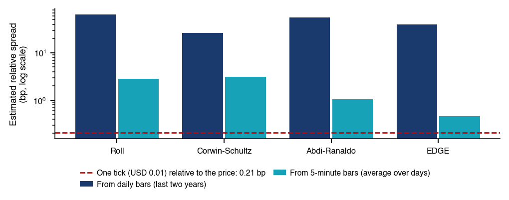

 MFM_ch10_order_book

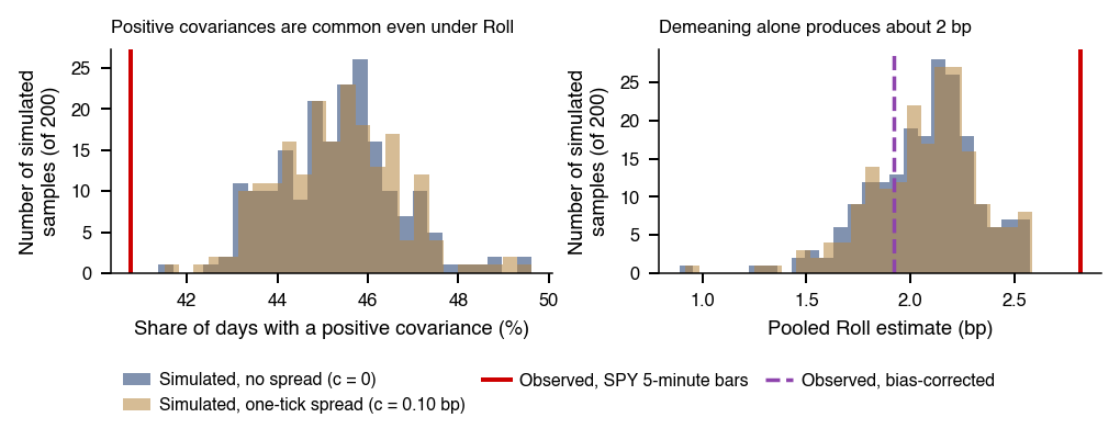
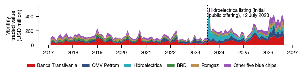
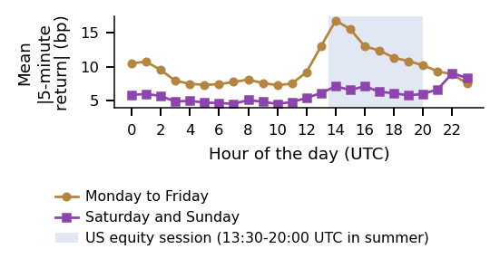
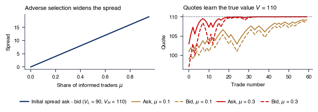
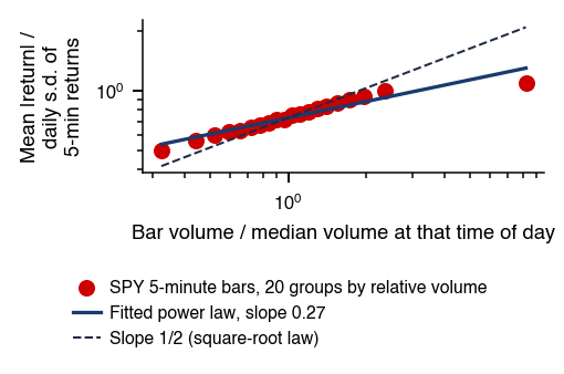
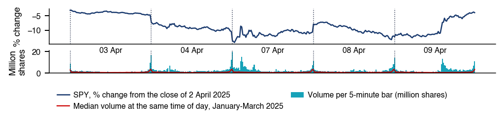
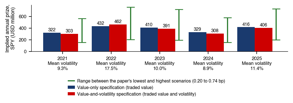


 Applied Computational Finance