Chapter 2: Market Efficiency — From EMH to Adaptive Markets
Daniel Traian PELE
Bucharest University of Economic Studies IDA Institute Digital Assets Blockchain Research Center AI4EFin Artificial Intelligence for Energy Finance Romanian Academy, Institute for Economic Forecasting MSCA Digital Finance
Can Past Prices and Public Information Predict Returns?
“A market in which prices always ‘fully reflect’ available information is called ‘efficient.’ ” — Fama (1970)
Lag-1 autocorrelation of daily returns: \(-0.099\) for the S&P 500 (Standard & Poor's) and \(0.109\) for the BET (Bucharest Exchange Trading, index), both significant
Bitcoin: \(-0.022\), inside the robust test band, so we do not reject \(\rho_1 = 0\)
Yesterday's return explains \(0.98\%\) of the variance of today's return for the S&P 500 and \(1.19\%\) for the BET
Dividend–price ratio, 680 monthly forecasts for the S&P 500: out-of-sample \(R^2 = -0.51\%\)
the forecast is worse than the historical mean
Of 2 000 random trading rules, \(5.2\%\) are “significant” at 5%
the best one has \(|t| = 3.30\), although it is pure chance
The chapter asks whether past prices, news or other public information can predict returns, after adjusting for risk and costs. The definition of Fama (1970) depends on the information set: the weak form of efficiency concerns past prices and returns, the semi-strong form all public information, and the strong form private information as well. Every test also needs a model of the expected return, so a rejection does not by itself prove inefficiency: this is the joint hypothesis problem.
Across 16 series of daily log returns, the lag-1 autocorrelation is positive and significant for the BET (0.109), IPC (0.071), Nifty 50 (0.048) and EUR (euro)/RON (0.170), and negative and significant for the S&P 500 (Standard & Poor's) (−0.099). For Bitcoin (−0.022) and Ethereum (−0.012) it stays inside the robust test band. The effect is small: yesterday's return explains 0.98% of the variance of today's return for the S&P 500 and 1.19% for the BET. The proposed mechanisms, infrequent trading, the managed-float regime and overreaction, are not tested here.
Out-of-sample forecasts and multiple testing call for the same caution. With the dividend–price ratio, the 680 monthly forecasts for the S&P 500 have an out-of-sample \(R^2\) of −0.51%, and the Clark–West test gives \(t = 0.42\), so we do not reject the absence of predictability. Of 2,000 random trading rules, 5.2% are “significant” at 5%, as the test level implies, and the best one has \(|t| = 3.30\), although it is pure chance. The number of rules tried matters as much as the threshold chosen.
Lag-1 autocorrelation, \(\hat\rho_1\), of daily log returns in 16 markets, each over its full sample: the bars are 95% confidence intervals with HAC (heteroskedasticity and autocorrelation consistent) standard errors, the light band is the robust test band around 0, and the dashes mark the i.i.d. band. Interactive chart: “Lag-1 Autocorrelation Across Markets (1/3)” →
What you will be able to do
Derive the random-walk restrictions and the variance ratio from the autocorrelations.
Compute the lag-1 autocorrelation and the variance ratio with robust standard errors.
Compute the out-of-sample \(R^2\) and the Clark–West test.
Compute the cumulative abnormal return in an event study.
Interpret an anomaly after the Holm correction.
The Further Topics and the Appendix are reading for familiarity.
Returns and informationEfficiency and the information set, the joint hypothesis problem and the random-walk models RW1 (Random Walk 1, i.i.d. increments)–RW3 (Random Walk 3, uncorrelated increments).
Topics for further studyData, rational bubbles, test construction, predictive regressions, long memory, event-study inference, behavioural anomalies and machine learning.
The chapter asks whether past prices, news or other public information can predict returns after adjusting for risk and costs. Sections 1 to 5 contain the core material, and each ends with a short check and its answers. The topics for further study then give the derivations, the remaining tests and the project topics; detailed examples and advanced topics are in Further Topics, after the synthesis.
derive the random-walk restrictions and the variance ratio
compute the lag-1 autocorrelation and the variance ratio robustly
compute the out-of-sample \(R^2\) and the Clark–West test
compute the cumulative abnormal return in an event study
interpret an anomaly after the Holm correction
Further Topics and Appendix: reading for familiarity
Returns and information
The section makes the statement "past prices contain no information" precise. Market efficiency is defined relative to an information set, and the weak, semi-strong and strong forms differ in what that set contains. Every test of efficiency also needs a model of expected returns, so a rejection is always a joint rejection. The section then sets out the random-walk model of log prices and its three versions, RW1, RW2 (Random Walk 2, independent increments) and RW3, which differ only in what they assume about the shocks, and shows with simulated series why the difference between zero correlation and independence matters for returns.
The random walk comes in three versions of decreasing strength:
RW1 (Random Walk 1) assumes independent and identically distributed increments;
RW2 keeps independence but lets the distribution change over time;
RW3 requires only that the increments be uncorrelated, so they may still be dependent.
The question of the section is what it means, precisely, that past prices contain no information about future returns.
The version matters for testing. A test built under RW1 can reject only because volatility varies over time, although the increments remain uncorrelated. A second difficulty is independent of the version: every test also needs a model of expected returns, so a rejection does not by itself prove that the market is inefficient.
In brief
RW1: Random Walk 1 — independent, identically distributed increments.
RW2: Random Walk 2 — independent increments, possibly with different distributions.
RW3: Random Walk 3 — uncorrelated increments, possibly dependent.
The question: what does it mean, precisely, that past prices contain no information?
information about future returns
Which random-walk version we test matters: a test built under RW1 can reject only because volatility varies over time.
Every test also needs a model of expected returns, so a rejection does not by itself prove inefficiency.
A Real Price Series among Simulated Random Walks (1/2)
Question for the room One of the four series is the S&P 500 from 2010 to 2026; the other three are random walks with the same drift and volatility. All four paths show trends and sharp falls. What can we infer from these features alone?
Answer
A random walk with drift can produce trends, and Normal innovations can produce large moves. These visual features alone do not constitute a statistical rejection. The real series is D; recognising it does not establish return predictability. This is why efficiency is tested with statistics rather than by inspection.
The chart shows four price paths. One of them is the S&P 500 (Standard & Poor's 500); the other three are simulated random walks. The reader is asked to pick the real market before the answer is given on the next slide.
In the interactive version, the slider moves the trading day along the four paths and the menu reveals the real series. The button "New random walks" draws three new simulated paths, so the game can be repeated with different pictures.
The real series is panel D. The point of the game is not whether the reader guessed it: Roberts (1959) showed that simulated random walks produce "patterns" by chance, trends and sharp falls that the eye reads as structure. Visual inspection therefore cannot separate a market from a random walk, and the chapter relies on statistical tests instead.
The economic argument goes back to Bachelier (1900) and Samuelson (1965): prices that are properly anticipated fluctuate randomly. If all the information about future cash flows is already in today's price, the next price change reflects only news, which cannot be foreseen. Unpredictability is then the mark of a well-functioning market, not of a disorderly one.
In brief
Which panel is the S&P 500? Vote: A, B, C or D?
<2-> Answer: D.
<2-> Roberts (1959): simulated random walks produce “patterns” by chance
<2-> We need statistical tests, not visual inspection
Fama (1970) defines a market as efficient if prices "fully reflect" all available information \(\mathcal{I}_t\); this is the Efficient Market Hypothesis (EMH). Formally, no strategy that uses \(\mathcal{I}_t\) earns expected returns above the fair, risk-adjusted return. The definition is about expected returns: a strategy may be lucky in a given sample without contradicting efficiency.
The definition depends on what \(\mathcal{I}_t\) contains. In the weak form it contains past prices and returns, and the typical tests are autocorrelations and variance ratios, with runs and long-memory tests in the appendix. In the semi-strong form it contains all public information, such as news and reports, and the typical test is the event study. In the strong form it contains private, insider information as well, and the tests look at the returns of insiders and fund managers.
The three forms are nested. The strong form implies the semi-strong form, which implies the weak form, because each information set contains the previous one. Adjusting returns for risk with factor models, which the fair return requires, is the subject of Chapter 3.
In brief
Fama (1970): a market is efficient if prices “fully reflect” all available information \(\mathcal{I}_t\)
The "fair return" in the definition of efficiency requires a model of expected returns, for example the Capital Asset Pricing Model (CAPM) of Chapter 3. Every test of efficiency is therefore a joint test of efficiency and of the asset-pricing model (Fama, 1991). A rejection may mean that the market is inefficient, or that the model of risk is wrong. Predictable expected returns are allowed in an efficient market if they compensate a risk that varies over time.
The problem is least severe at short horizons. At daily horizons expected returns are tiny, so the choice of model matters little, and weak-form tests on daily data are the cleanest tests of efficiency. The logic of testing also limits what can be concluded: efficiency can never be "proved", only not rejected by a given test on given data.
In brief
CAPM: Capital Asset Pricing Model.
“Fair return” requires a model of expected returns
"The past contains no information" can mean two different things: zero correlation or independence. The lag-\(k\) autocorrelation is the correlation between a return and the return \(k\) periods earlier. Zero correlation excludes a linear association between the two, but it may leave dependence in nonlinear functions of the returns, for example in their squares.
A toy example shows the gap. Let \(X\) take the values \(-2, -1, 1, 2\) with equal probability and let \(Y = X^2\). Then \(\mathbb{E}[X] = 0\) and \(\mathbb{E}[XY] = (-8-1+1+8)/4 = 0\), so the covariance and the correlation are zero. Yet knowing \(X\) determines \(Y\) exactly: the two variables are as dependent as variables can be. For returns, the analogue is a series whose levels are uncorrelated while the sizes of the moves, measured by squared returns, are dependent.
Let \(P_t\) be the index level at the close of day \(t\) and \(p_t = \ln P_t\) the log price. The random walk with drift is
\[p_t = \mu + p_{t-1} + \varepsilon_t,\]
(2.1)
where \(\mu\) is the drift, the mean growth per day, and \(\varepsilon_t\) is the day's shock, with mean zero and variance \(\sigma^2\). By repeated substitution, \(p_t = p_0 + \mu t + \sum_{s=1}^{t}\varepsilon_s\): the log price is a linear trend plus the sum of all past shocks. Equivalently, the log return is \(r_t = p_t - p_{t-1} = \mu + \varepsilon_t\).
With the information set \(\mathcal{I}_t = \{p_t, p_{t-1}, \dots\}\), the best forecast of the future log price is \(\mathbb{E}[p_{t+h} \mid \mathcal{I}_t] = p_t + \mu h\), today's price plus the drift. This holds if the shocks have conditional mean zero, \(\mathbb{E}[\varepsilon_{t+1} \mid \mathcal{I}_t] = 0\). Zero autocorrelations alone (RW3) are not enough: under RW3 the past does not, in general, improve the best linear forecast, but a nonlinear function of the past may still help.
If the shocks are uncorrelated with variance \(\sigma^2\), the variance of the \(h\)-day change is \(\mathrm{Var}(p_{t+h} - p_t) = h\,\sigma^2\): it grows linearly with the horizon. This property is the basis of the variance ratio in section 2. RW1, RW2 and RW3 differ only in what they assume about the shocks \(\varepsilon_t\)(Campbell, Lo & MacKinlay, 1997).
The three versions of the random walk are distinguished by the condition imposed on the shocks:
Under RW1, the shocks are independent and identically distributed (i.i.d.), with mean 0 and variance \(\sigma^2\); an illustrative model is \(r_t = \mu + 0.01 z_t\), with \(z_t\) i.i.d. with the standard Normal distribution \(N(0,1)\).
Under RW2, the shocks are independent but their variance \(\sigma_t^2\) may vary over time; the illustration is \(r_t = \mu + \sigma_t z_t\), with \(\sigma_t\) equal to 1% and then 3%, fixed in advance.
Under RW3, only \(\mathrm{Cov}(\varepsilon_t, \varepsilon_{t-k}) = 0\) for every \(k \ge 1\) is required.
The example of RW3 used throughout the chapter is the GARCH (Generalized AutoRegressive Conditional Heteroskedasticity) model,
in its GARCH(1,1) form, with \(\omega > 0\) and \(\alpha, \beta \ge 0\). Today's variance depends on yesterday's squared shock and yesterday's variance.
The versions are nested. RW1 implies RW2, because i.i.d. returns are in particular independent; RW2 implies RW3, because independent returns are in particular uncorrelated, provided their variance exists. A GARCH model keeps zero correlation but violates RW2: the size of today's move depends on past shocks. And RW3 does not make tomorrow's mean unpredictable, since a nonlinear function of the past can forecast it.
The chart shows three simulated series with mean zero, one for each version of the random walk: daily returns at the top and, below, the conditional standard deviation (SD) used in the simulation. The RW2 volatility is fixed in advance, 1% and then 3% from the middle of the sample, while the GARCH volatility responds to past shocks.
In the interactive version, the sliders set the GARCH parameters \(\alpha\), the reaction to yesterday's shock, and \(\beta\), the persistence of the variance, as well as the RW2 volatility after day 450. The ▶ button changes the parameter step by step.
Question for the room RW2 has independent returns, with standard deviation 1% up to day 450 and 3% after; GARCH has turbulent periods after large shocks. What is the kurtosis of RW2 in this simulation?
Answer
Clearly above 3: 4.8, against 3.0 for RW1 and 4.1 for GARCH. Mixing a calm period with a turbulent one gives fat tails without any dependence, so neither the chart of returns nor the kurtosis tells RW2 from GARCH. The difference lies elsewhere: in RW2 volatility rises at a date fixed in advance and the returns stay independent; in GARCH today's volatility depends on yesterday's shock (α = 0.08) and on yesterday's volatility (β = 0.90), so the returns are dependent.
The GARCH series shows volatility clustering: large moves tend to be followed by large moves. The RW2 series also has a turbulent period, although its returns are independent. The chart alone therefore cannot tell a regime change fixed in advance from volatility clustering; the difference lies in whether volatility depends on past shocks.
In brief
SD: Standard Deviation.
Three simulated series with mean zero.
daily returns on top; below, the conditional standard deviation used in the simulation.
RW2 volatility is fixed in advance, while GARCH volatility responds to past shocks.
1% then 3%, from the middle of the sample.
Volatility clustering: large moves tend to be followed by large moves.
The RW2 series also has a turbulent period although its returns are independent.
The chart alone cannot tell a regime change fixed in advance from volatility clustering.
The chart compares two autocorrelation functions of the same simulated GARCH series. On the left are the autocorrelations of the returns, on the right those of the squared returns, at lags up to 20.
In the interactive version, the sliders set \(\alpha\) and \(\beta\), and the menu sets the length \(T\) of the series, from 900 to 10,000 days.
Question for the room Keep β = 0.90 and the 900-day series. As α rises from 0.08 to 0.095, how does the sample lag-1 autocorrelation of squared returns change?
Answer
It rises: in this simulation, the sample autocorrelation rises from 0.216 to 0.272. A long-run variance of 1 does not fix the dependence of squared returns. At α = 0.095, 3α² + 2αβ + β² equals 1.0081: the stationary model has no finite fourth moment, so the theoretical ACF of squared returns is undefined. The sample ACF of the finite series can still be calculated. At α = 0 the returns are independent: the sample autocorrelation of the squares is 0.049 at lag 1 and goes down to −0.050 over lags 1–20. For α > 0 the series satisfies RW3 but violates RW2: the size of today's move depends on past shocks.
The autocorrelations of the returns are close to zero at all lags, as RW3 requires. The autocorrelations of the squared returns are positive up to lag 20: a day with a large move is followed by other days with large moves. This is the toy example of zero correlation with dependence, now in a model of returns.
In brief
Left: the autocorrelations of simulated GARCH returns are close to zero at all lags.
Right: the autocorrelations of squared returns are positive up to lag 20.
a day with a large move is followed by other days with large moves.
The three questions test the distinctions of the section: between RW1 and RW2, between zero autocorrelation and independence, and between rejecting a test and proving inefficiency.
In brief
Can returns remain independent if their standard deviation moves from 1% to 3% on a date fixed in advance?
Does zero autocorrelation establish independence?
Why does rejecting an efficiency test not, on its own, prove that the market is inefficient?
Returns can remain independent when their standard deviation moves from 1% to 3% on a date fixed in advance: the series satisfies RW2 but violates RW1, because the distribution is no longer identical over time. Zero autocorrelation does not establish independence; in the GARCH example the returns are uncorrelated while their squares are dependent. Finally, a rejection does not on its own prove inefficiency, because every test of efficiency also tests the model of expected returns, and a wrong risk model can produce the rejection.
In brief
Yes. The series satisfies RW2 but violates RW1, because the distribution is no longer identical.
No. In the GARCH example, return autocorrelation is zero, but squared returns are dependent.
Every efficiency test also tests the model of expected returns.
A rejection can come from a wrong risk model (the joint-hypothesis problem).
Section summary
Efficiency is a statement about an information set and about expected returns, and it can be tested only jointly with a model of risk. For the weak form, the three versions of the random walk separate zero correlation from independence: RW3, the weakest, allows the volatility clustering seen in returns. The next section tests RW3 with autocorrelations and variance ratios whose standard errors remain valid under such clustering.
Autocorrelation and variance ratios
The section tests the weak form on 16 daily series: 13 stock indices, Bitcoin, Ethereum and the EUR/RON reference rate. The first statistic is the lag-1 autocorrelation, the second the variance ratio, which accumulates the autocorrelations up to a horizon of \(q\) days. Both are tested with standard errors that remain valid when volatility clusters, and the multiplicity of horizons is handled by the Chow–Denning test.
The question of the section is whether today's return predicts tomorrow's, in equity, crypto and currency markets. The lag-1 autocorrelation \(\rho_1\) measures the linear dependence between consecutive days, and the variance ratio accumulates the autocorrelations up to horizon \(q\).
The markets are 13 stock indices, developed and emerging, including the BET, together with Bitcoin, Ethereum and the EUR/RON reference rate. The selection includes markets where predictability is more likely: where liquidity is thin, as for the BET and the crypto-assets, or where the exchange rate is managed, as for EUR/RON. All samples end on 18 September 2026. The equity series start in January 2000, EUR/RON in July 2005, Bitcoin in September 2014 and Ethereum in January 2016.
In brief
The question: does today's return predict tomorrow's in equity, crypto and currency markets?
The lag-1 autocorrelation \(\rho_1\) measures linear dependence between consecutive days.
The variance ratio accumulates the autocorrelations up to horizon \(q\).
Markets: 13 stock indices, Bitcoin, Ethereum and the EUR (euro)/RON reference rate.
developed and emerging, including the BET.
Why this selection: predictability is more likely:
where liquidity is thin (BET, crypto).
or where the exchange rate is managed (EUR/RON).
Samples: all to 18 September 2026.
equities from January 2000, EUR/RON from July 2005.
Bitcoin from September 2014 and Ethereum from January 2016.
The chart shows, for each of the 16 markets, the lag-1 autocorrelation \(\hat\rho_1\) of daily log returns over its full sample, with its 95% confidence interval. Around zero, two bands serve for testing: the robust test band and the narrower band implied by i.i.d. returns. The next slide explains how they are built and how to read them.
In the interactive version, the slider changes the lag \(k\) from 1 to 10, and the ▶ button runs through the lags.
Question for the room In a hypothetical example, the estimated autocorrelation is −0.040, the i.i.d. standard error is 0.012, and the robust standard error under H₀ is 0.027. Using the asymptotic two-sided cutoff of 1.96, which test rejects H₀: ρ₁ = 0?
Answer
Only the test using the i.i.d. standard error. With the i.i.d. standard error, |z| = 0.040/0.012 = 3.33; with the robust error, |z| = 0.040/0.027 = 1.48. The decision depends on the estimate relative to its standard error, not on the autocorrelation's magnitude alone. For the S&P 500, ρ̂₁ = −0.099 lies outside both test bands, with the same standard errors (0.027 robust, 0.012 i.i.d.); for the Euro Stoxx 50 or the Nikkei 225, ρ̂₁ falls outside the i.i.d. band but inside the robust one. The bars around the estimates are confidence intervals with the HAC standard error of the estimator (S&P 500: 0.030); they serve for comparisons, not for the test of ρ₁ = 0.
The rule for reading the chart is to compare each dot with the robust band, not with the i.i.d. band and not with the confidence interval. The markets whose dots lie outside the robust band are listed on the third slide.
Each dot is the lag-1 autocorrelation \(\hat\rho_1\) of one market's daily log returns. The coloured bar is the 95% confidence interval \(\hat\rho_1 \pm 1.96\,\mathrm{SE}_{\mathrm{HAC}}\), where \(\mathrm{SE}_{\mathrm{HAC}}\) is the heteroskedasticity and autocorrelation consistent (HAC) standard error of the estimator, valid also when \(\rho_1 \neq 0\). The light band is the robust test band \(0 \pm 1.96\,\mathrm{SE}_0\), where \(\mathrm{SE}_0\) is derived under the null hypothesis \(H_0\) of an unpredictable mean. The ticks mark the i.i.d. band \(0 \pm 1.96/\sqrt{T}\), where \(T\) is the number of daily returns.
The test and the interval answer different questions, and they can disagree. We reject \(\rho_1 = 0\) at 5% if the dot lies outside the robust test band. For the Nikkei 225 and the PX, the HAC interval excludes 0, but \(\hat\rho_1\) stays inside the test band, so we do not reject.
The i.i.d. band is too narrow under volatility clustering. In all 16 series, \(\mathrm{SE}_0\) exceeds the i.i.d. value; for the S&P 500, with \(T = 6\,717\) daily returns, it is 0.027 against 0.012. The abbreviations BIST (Borsa İstanbul, BIST 100 index, the Istanbul Stock Exchange, BIST 100 index), WIG20 (Warszawski Indeks Giełdowy 20, the Warsaw Stock Exchange index of the 20 largest companies), BUX (Budapesti Értéktőzsde index, the Budapest Stock Exchange index), PX, IPC and BET denote the stock-exchange indices of Istanbul, Warsaw, Budapest, Prague, Mexico and Bucharest, and FX (foreign exchange) denotes the EUR/RON reference rate.
In brief
SE: Standard Error; HAC: Heteroskedasticity and Autocorrelation Consistent; CI: Confidence Interval.
Each dot is the lag-1 autocorrelation \(\hat\rho_1\) of one market's daily log returns, over its full sample.
The coloured bar is the 95% confidence interval \(\hat\rho_1 \pm 1.96\,\text{SE}_{\text{HAC}}\).
\(\text{SE}_{\text{HAC}}\): the standard error of the estimator, valid also when \(\rho_1 \neq 0\) (formula).
The light band is the robust test band \(0 \pm 1.96\,\text{SE}_0\); the ticks mark the i.i.d. band \(0 \pm 1.96/\sqrt{T}\).
\(\text{SE}_0\): derived under \(H_0\) (unpredictable mean), test construction; \(T\): the number of daily returns.
Reading rule: we reject \(\rho_1 = 0\) at 5% if the dot lies outside the robust test band.
Nikkei 225 and PX (the Prague Stock Exchange index): the HAC interval excludes 0, but \(\hat\rho_1\) stays inside the test band, so we do not reject.
In all 16 series, \(\text{SE}_0\) exceeds the i.i.d. value; for the S&P 500 (\(T = 6\,717\)) it is \(0.027\) against \(0.012\).
BIST (Borsa İstanbul, BIST 100 index), WIG20 (Warszawski Indeks Giełdowy 20, the 20 largest companies), BUX (Budapesti Értéktőzsde index), PX, IPC (Índice de Precios y Cotizaciones) and BET: the stock indices of Istanbul, Warsaw, Budapest, Prague, Mexico and Bucharest.
FX is foreign exchange (the EUR/RON reference rate).
Four series have positive and significant autocorrelations: the BET (\(\hat\rho_1 = 0.109\)), the IPC (0.071), the Nifty 50 (0.048) and EUR/RON (0.170). The S&P 500 has a negative and significant autocorrelation, \(\hat\rho_1 = -0.099\). For Bitcoin (\(-0.022\)) and Ethereum (\(-0.012\)) the estimates lie inside the robust test band, so we do not reject \(\rho_1 = 0\).
The slide proposes a mechanism for each finding. For the BET, persistence can come from thin trading in some stocks, whose prices absorb news with a delay. For EUR/RON, it can come from the managed float, in which the central bank smooths exchange-rate moves. For the S&P 500, the reversal can come from short-term overreaction and liquidity provision. These mechanisms are not tested here: what the result supports is description.
The effects are also small. The square \(\hat\rho_1^2\), the share of today's return variance explained by yesterday's return, is 0.98% for the S&P 500 and 1.19% for the BET. Both robust standard errors require a finite fourth moment of returns, an assumption that Chapter 1 questions.
In brief
BET (\(\hat\rho_1 = 0.109\)), IPC (\(0.071\)), Nifty 50 (\(0.048\)) and EUR/RON (\(0.170\)): positive and significant autocorrelations.
S&P 500: \(\hat\rho_1 = -0.099\), negative and significant.
Bitcoin (\(\hat\rho_1 = -0.022\)) and Ethereum (\(-0.012\)): inside the robust test band, so we do not reject \(\rho_1 = 0\).
For the BET, persistence can come from thin trading in some stocks, whose prices absorb news with a delay.
For EUR/RON, it can come from the managed float, in which the central bank smooths exchange-rate moves.
For the S&P 500, the reversal can come from short-term overreaction and liquidity provision.
The effect is small: \(\hat\rho_1^2\) is \(0.98\%\) for the S&P 500 and \(1.19\%\) for the BET.
the share of today's return variance explained by yesterday's return.
Both robust standard errors require a finite fourth moment, which Chapter 1 questions.
Type of evidence: description (it shows what happened in the data, without testing a cause).
The proposed mechanisms (thin trading, managed float, overreaction) are not tested here.
The lag-1 autocorrelation looks at a single lag. Small autocorrelations at many lags can each pass the test and still accumulate over longer horizons. The variance ratio (VR) of Lo & MacKinlay (1988) measures this accumulation. Over a horizon of \(q\) days,
the variance of the \(q\)-day return divided by \(q\) times the variance of the daily return; \(q = 5\) is one trading week. Without autocorrelation, the variance grows linearly with the horizon, as in the random-walk model, and \(\mathrm{VR}(q) = 1\). The estimate \(\widehat{\mathrm{VR}}(q)\) tends to 1 even when volatility varies over time, as under RW2 and RW3.
For a covariance-stationary series, the ratio is a weighted sum of autocorrelations,
with weights that fall with the lag \(k\). A value \(\mathrm{VR}(q) > 1\) signals persistence, a value below 1 reversal (mean reversion). For \(q = 2\),(2.4) gives \(\mathrm{VR}(2) = 1 + \rho_1\): on the S&P 500, \(1 - 0.099 = 0.901\), equal to \(\widehat{\mathrm{VR}}(2)\) estimated directly from (2.3).
In brief
VR: Variance Ratio.
Why another test: \(\hat\rho_1\) looks at a single lag.
small autocorrelations at many lags can each pass the test yet accumulate over longer horizons.
Variance ratio over a horizon of \(q\) days Lo & MacKinlay (1988): \(\text{VR}(q) = \dfrac{\Var(r_t + \dots + r_{t-q+1})}{q\,\Var(r_t)}\).
equal to 1 without autocorrelation.
\(q = 5\): one trading week.
Without autocorrelation, \(\widehat{\text{VR}}(q)\) tends to 1 even when volatility varies over time (RW2, RW3).
For a covariance-stationary series, \(\text{VR}(q) = 1 + 2 \sum_{k=1}^{q-1} \big(1 - \tfrac{k}{q}\big) \rho_k\).
a weighted sum of autocorrelations, with weights that fall with the lag \(k\).
The test of the variance ratio uses a band centred at 1, the value under the null. With \(T\) daily returns, the robust 95% null band is
\[1 \pm 1.96\sqrt{\hat\theta(q)/T},\]
(2.5)
where \(\hat\theta(q)\) is the estimated variance of \(\sqrt{T}\,(\widehat{\mathrm{VR}}(q) - 1)\), robust to heteroskedasticity. If \(\widehat{\mathrm{VR}}(q)\) falls outside the band, we reject the null at 5%.
The band is not a confidence interval: a confidence interval would be centred at the estimate \(\widehat{\mathrm{VR}}(q)\), not at 1. Its width responds to two features of the data. When large moves follow large moves (volatility clustering), \(\hat\theta(q)\) grows and the band widens. \(\hat\theta(q)\) also grows with \(q\), so the band widens at long horizons, because a sample contains fewer independent \(q\)-day periods.
In brief
The robust 95% band is centred at 1, the value under the null.
if \(\widehat{\text{VR}}(q)\) falls outside it, we reject the null at 5%.
The band is not a confidence interval.
a confidence interval would be centred at the estimate \(\widehat{\text{VR}}(q)\), not at 1.
The robust null band is \(1 \pm 1.96\sqrt{\hat\theta(q)/T}\) (test construction).
\(T\): the number of daily returns.
\(\hat\theta(q)\): the estimated variance of \(\sqrt{T}\,(\widehat{\text{VR}}(q) - 1)\), robust to heteroskedasticity.
When large moves follow large moves (volatility clustering), \(\hat\theta(q)\) grows and the band widens.
\(\hat\theta(q)\) also grows with \(q\), so the band widens at long horizons.
a sample contains fewer independent \(q\)-day periods.
Reversal or persistence can appear at one day, a week or a month, and we do not know in advance at which. The chapter tests four horizons, \(q = 2, 5, 10, 20\) trading days: two days, about one week, two weeks and one trading month. The choice follows Lo & MacKinlay (1988), who use \(q = 2, 4, 8, 16\) on weekly data; other horizons can give a different result.
The robust null band (2.5) has level 5% at each horizon separately. With four tests, a false rejection occurs more often than 5% of the time. The Chow–Denning test (Chow & Denning, 1993) corrects this by using the largest robust statistic \(|z^*(q)|\) across the four horizons, with a critical value of 2.49 instead of 1.96.
With this correction, the test rejects RW3 for 5 of the 16 series, including the BET and the S&P 500. For Bitcoin it does not reject RW3 (p-value 0.835). Like the autocorrelation test, \(z^*\) and the Chow–Denning test require a finite fourth moment, which Chapter 1 questions.
In brief
Why several horizons: reversal or persistence can appear at one day, a week or a month.
we do not know in advance at which.
We test four horizons, \(q = 2, 5, 10, 20\) trading days.
two days, about one week, two weeks and one trading month.
The choice follows Lo & MacKinlay (1988), who use \(q = 2, 4, 8, 16\) on weekly data.
other horizons can give a different result.
The robust null band has level 5% at each horizon separately.
with four tests, a false rejection occurs more often than 5% of the time.
The chart shows the variance-ratio profile of several markets: the estimated \(\widehat{\mathrm{VR}}(q)\) as a function of the horizon \(q\), with the robust 95% band around 1.
In the interactive version, the menu chooses the group of markets (the four markets of the slide, Central and Eastern Europe, developed markets, or emerging markets with Ethereum), and the slider sets the horizon \(q\) from 2 to 60 days.
Question for the room For the S&P 500, the 20-day variance ratio is 0.754. For this value, what is the standard-error boundary below which |(VR − 1)/SE| exceeds 1.96?
Answer
The boundary is |0.754 − 1|/1.96 = 0.1255. The value 0.2460 is the deviation from the null before division by the cutoff. The value 0.1328 is the actual robust standard error at 20 days; it exceeds the boundary, so the test does not reject. The null band widens with q: its lower edge is 0.817 at 10 days, where VR = 0.767 is rejected, and 0.740 at 20 days. The calculation uses overlapping aggregated returns and the robust Lo–MacKinlay standard error.
A profile above the band signals persistence that accumulates with the horizon, a profile below it reversal. The band widens with \(q\), so a deviation of the same size is less significant at long horizons; the values for each market are on the next slide.
Each curve shows \(\widehat{\mathrm{VR}}(q)\) for horizons from 2 to 60 days; the horizon of 60 days, about three trading months, is only descriptive. The shaded area is the robust 95% band around 1.
For the S&P 500 the profile lies below 1, a reversal, and leaves the band at 2, 5 and 10 days: \(\widehat{\mathrm{VR}}(2) = 0.901\),\(\widehat{\mathrm{VR}}(5) = 0.829\) and \(\widehat{\mathrm{VR}}(10) = 0.767\). At 20 days it is just inside the band, \(0.754\) against the edge \(0.740\); at 60 days it is \(0.674\). For the BET the profile lies above 1, a persistence that rises with \(q\), and leaves the band at all four tested horizons: \(\widehat{\mathrm{VR}}(2) = 1.108\),\(\widehat{\mathrm{VR}}(5) = 1.173\),\(\widehat{\mathrm{VR}}(10) = 1.225\) and \(\widehat{\mathrm{VR}}(20) = 1.377\), with \(1.644\) at 60 days.
Bitcoin stays inside the band at all horizons, so the null is not rejected. For EUR/RON the ratio stays above 1 at every horizon but leaves the band only at 2 and 5 days, with \(\widehat{\mathrm{VR}}(2) = 1.170\) and \(\widehat{\mathrm{VR}}(5) = 1.157\). As for the autocorrelations, what the result supports is description.
In brief
Each curve shows the estimated variance ratio \(\widehat{\text{VR}}(q)\) for horizons \(q\) from 2 to 60 days.
\(q = 60\), about three trading months, is only descriptive.
The shaded area is the robust 95% band around 1, the value without autocorrelation.
S&P 500: \(\widehat{\text{VR}}(q)\) is below 1 (reversal) and leaves the band at 2, 5 and 10 days
at 20 days it is just inside the band: \(0.754\) against the edge \(0.740\)
The questions concern the standard error under volatility clustering, the gap between statistical and economic significance, the meaning of a variance ratio below one, and a transfer exercise in which the standard error of a variance-ratio estimate doubles.
In brief
Why can an i.i.d. band be misleading under volatility clustering?
Does positive autocorrelation imply profit after costs?
What does a variance ratio below one suggest?
Transfer: a test statistic has magnitude 2.4.
If the VR estimate stays the same but its standard error doubles, what does the magnitude become?
Under volatility clustering, the i.i.d. standard error ignores the dependence in squared returns, so it is too small and the test rejects the null too often. A positive autocorrelation does not imply profit after costs: effect size, risk, implementation and costs still matter. A variance ratio below 1 suggests reversal over the chosen horizon, and calling the deviation significant requires a robust standard error. In the transfer exercise, a statistic of magnitude 2.4 halves to 1.2 when the standard error doubles; 1.2 does not cross 1.96, so the null is no longer rejected. The estimated effect is unchanged; only the evidence for it is weaker.
In brief
The i.i.d. standard error ignores dependence in squared returns, so it is too small.
The test rejects the null too often.
No: effect size, risk, implementation and costs still matter.
A variance ratio below 1 suggests reversal over the chosen horizon.
To call the deviation significant, we need a robust standard error.
The statistic halves to 1.2.
No: 1.2 does not cross 1.96.
the estimated effect is unchanged, its evidence is weaker.
Section summary
Four of the 16 series have a significant positive lag-1 autocorrelation and the S&P 500 a significant negative one, while Bitcoin and Ethereum stay inside the robust band. The variance-ratio profiles confirm reversal on the S&P 500 and persistence on the BET over several horizons. The effects are small, and the proposed mechanisms are not tested. The next section asks a different question: whether a predictor forecasts returns on data not used to estimate it.
Out-of-sample predictability
The section moves from the dependence of returns on their own past to forecasting with another variable, the log dividend–price ratio. The test is out of sample: each forecast uses only the data available when it is made, and it is scored against the historical mean with the out-of-sample \(R^2\) and the Clark–West test.
The question is whether a variable known today forecasts next month's market return. The classic candidate is \(dp\), the log dividend–price ratio: dividends over the last 12 months divided by the average index level in that month.
In sample, regressions of returns on such variables appear to work. On new data, most published predictors fail (Welch & Goyal, 2008). The proper test is therefore one in which every forecast uses only the data available when it is made.
In brief
The question: does a variable known today forecast next month's market return?
The classic candidate is \(dp\), the log dividend–price ratio.
dividends over the last 12 months divided by the average index level in that month.
Let \(r\) be the monthly S&P 500 log return, with dividends, minus the 3-month US (United States) Treasury bill rate. Each month \(t\), the predictive regression
\[r_{s+1} = \alpha + \beta\, dp_s + u_{s+1}\]
(2.6)
is estimated on all months up to \(t\); at the next step the window grows by one month (an expanding window). The out-of-sample (OS) forecast for month \(t+1\) is \(\hat r_{t+1} = \hat\alpha + \hat\beta\, dp_t\).
The competing forecast is the historical mean \(\bar r_{t+1}\), the mean of the returns up to month \(t\), which corresponds to no predictability. The first forecast is for January 1970, which gives 680 monthly forecasts.
One qualification applies. Monthly dividends are interpolated from quarterly totals, so \(dp_t\) was not known exactly in month \(t\), and the exercise is pseudo-out-of-sample.
In brief
OS: Out-of-Sample.
\(r\): the monthly S&P 500 log return, with dividends, minus the 3-month US (United States) Treasury bill rate.
Each month \(t\) we estimate \(r_{s+1} = \alpha + \beta\, dp_s + u_{s+1}\) on all months up to \(t\) (\(\alpha\), \(\beta\): intercept and slope, not the GARCH parameters).
at the next step the window grows by one month (expanding window).
The \(dp\) forecast for month \(t+1\): \(\hat r_{t+1} = \hat\alpha + \hat\beta\, dp_t\).
The competing forecast: the historical mean \(\bar r_{t+1}\).
The mean of returns up to month \(t\).
it corresponds to no predictability.
The first forecast is for January 1970, giving 680 monthly forecasts.
Monthly dividends are interpolated from quarterly totals.
with the sums over the forecast months. A positive \(R^2_{OS}\) means that the \(dp\) forecast has smaller squared errors than the historical mean; a negative one, that the historical mean forecasts better. Unlike the in-sample \(R^2\),\(R^2_{OS}\) can be negative.
The two measures differ because, in sample, \(\hat\beta\) also fits the noise of the months it explains. A positive \(R^2_{OS}\) can also arise by chance, so its significance is tested separately, with the Clark–West test reported in the results.
In brief
\(R^2_{OS} = 1 - \sum_t (r_t - \hat r_t)^2 \big/ \sum_t (r_t - \bar r_t)^2\), with the sums over the forecast months.
\(R^2_{OS} > 0\): the \(dp\) forecast has smaller squared errors than the historical mean.
\(R^2_{OS} < 0\): the historical mean forecasts better.
unlike the in-sample \(R^2\), \(R^2_{OS}\) can be negative.
Why the two differ: in sample, \(\hat\beta\) also fits the noise of the months it explains.
A positive \(R^2_{OS}\) can also arise by chance.
we test its significance separately (the Clark–West test, in the results).
The chart of the next slide accumulates the difference between the two forecasts month by month. Each month from 1970 adds \((r_t - \bar r_t)^2 - (r_t - \hat r_t)^2\), the squared error of the historical mean minus that of the \(dp\) forecast.
The curve therefore rises in months in which \(dp\) forecasts better and falls in months in which it forecasts worse, and its final value has the sign of \(R^2_{OS}\) in (2.7). On the vertical axis is the running sum, with returns as fractions (0.01 = 1%), squared.
In brief
Each month from 1970 adds \((r_t - \bar r_t)^2 - (r_t - \hat r_t)^2\).
the squared error of the historical mean minus that of the \(dp\) forecast.
The curve rises in months in which \(dp\) forecasts better and falls in months in which it forecasts worse.
The final value of the curve has the sign of \(R^2_{OS}\).
Vertical axis: the running sum, with returns as fractions (0.01 = 1%), squared.
The chart shows the cumulative difference of squared errors between the historical mean and the \(dp\) forecast for the S&P 500, month by month from 1970.
In the interactive version, the slider sets the year in which the evaluation starts, from 1970 to 2015, and the menu switches between the unrestricted \(dp\) forecast and the forecast with the Campbell–Thompson restrictions.
Question for the room Over 680 monthly forecasts from 1970, R²OS is −0.51%. Does it turn positive if the evaluation starts later?
Answer
No. For every start between 1970 and 2015, R²OS stays negative: −1.37% from 1990, −0.01% from 2000, −2.75% from 2010. The curve rises until 1990, and the 1990s boom wipes out the advantage. The Clark–West test over 1970–2026 gives t = 0.42 (p = 0.34), so the absence of predictability is not rejected.
The value at the right edge of the curve has the sign of \(R^2_{OS}\), and the slopes of the curve show in which periods \(dp\) helped or hurt. The results for the full sample are on the next slide.
The curve ends below zero: over the 680 monthly forecasts, \(R^2_{OS} = -0.51\%\). The historical mean forecast better than the \(dp\) regression over the whole evaluation period.
The Clark–West test (Clark & West, 2007) compares the squared errors and corrects a handicap of the \(dp\) model: even if \(\beta = 0\), estimating \(\beta\) adds noise to the forecast. On the S&P 500 the test gives \(t = 0.42\), with a one-sided p-value of 0.34, so we do not reject the absence of predictability. The test on squared errors requires a finite fourth moment, which Chapter 1 questions.
The path of the curve shows when the relation worked. Until 1990 the curve rises: \(dp\) forecast better than the historical mean. In the 1990s boom, \(dp\) fell to record lows while prices kept rising, and the advantage was lost. In the 2000s it partly returned, and after 2010 it was lost again. What the result supports is a comparison of procedures.
In brief
The curve ends below zero: over 680 monthly forecasts, \(R^2_{OS} = -0.51\%\).
The Clark–West test Clark & West (2007) compares the squared errors and corrects a handicap of the \(dp\) model.
even if \(\beta = 0\), estimating \(\beta\) adds noise to the forecast.
On the S&P 500 the test gives \(t = 0.42\) (one-sided \(p = 0.34\)).
we do not reject the absence of predictability.
the test on squared errors requires a finite fourth moment, which Chapter 1 questions.
Until 1990 the curve rises: \(dp\) forecast better than the historical mean.
In the 1990s boom, \(dp\) fell to record lows while prices kept rising: the advantage was lost.
In the 2000s the advantage partly returned, and after 2010 it was lost again.
Type of evidence: comparison of procedures (it shows which method works better on the same data, not why).
The Dividend–Price Ratio: Results for the S&P 500 (2/2)
A small \(R^2_{OS}\) can still matter economically. Campbell & Thompson (2008) show that even 0.5% is a lot for an investor: a mean–variance investor who raises equity exposure when the forecast is high and cuts it when it is low would raise the expected return by about 20%. The calculation uses the monthly market Sharpe ratio, 0.160; the formula is in the appendix.
Campbell and Thompson also impose two restrictions on the forecast: \(\hat\beta\) must have the sign that theory predicts, and the forecast of the equity premium must be non-negative. On the S&P 500 the restrictions bind in 5.7% of months and leave \(R^2_{OS}\) at \(-0.51\%\), so the economic gain is absent.
In brief
Does a small \(R^2_{OS}\) matter economically? Campbell & Thompson (2008) show that it does: even 0.5% is a lot for an investor.
A mean–variance investor would raise the expected return by about 20%.
who raises equity exposure when the forecast is high and cuts it when it is low.
The questions ask what a negative \(R^2_{OS}\) means, why a regression with a good in-sample fit can fail on new data, whether a profitable strategy can have a negative \(R^2_{OS}\), and what the loss of the \(dp\) advantage in the 1990s says about the stability of the relation.
In brief
What does a negative \(R^2_{OS}\) mean?
Why can a regression with a good in-sample \(R^2\) fail on new data?
Can a profitable strategy have a negative \(R^2_{OS}\)?
What does the loss of the \(dp\) advantage in the 1990s say about the stability of the relation?
A negative \(R^2_{OS}\) means that the historical mean forecast better than the model over the months evaluated. A regression with a good in-sample \(R^2\) can fail on new data because, in sample, \(\hat\beta\) also fits the noise, and on new data the noise does not repeat. A profitable strategy can have a negative \(R^2_{OS}\): its profit can come from constant market exposure or from a few correct sign calls, not from small squared errors. The loss of the advantage in the 1990s shows that the relation is not stable: a predictor that was useful until 1990 lost all its advantage when \(dp\) fell to record lows.
In brief
The historical mean forecast better than the model over the months evaluated.
In sample, \(\hat\beta\) also fits the noise.
on new data the noise does not repeat.
Yes: profit can come from constant market exposure or from a few correct sign calls.
not from small squared errors.
The relation is not stable.
a predictor that was useful until 1990 loses all its advantage when \(dp\) falls to record lows.
Section summary
On 680 monthly forecasts since 1970, the dividend–price ratio does not beat the historical mean for the S&P 500: \(R^2_{OS}\) is negative and the Clark–West test does not reject the absence of predictability. The relation worked until 1990 and was unstable afterwards. The next section turns to the semi-strong form and asks how prices react to a specific public announcement.
Event studies
The autocorrelation and predictability tests of the previous sections use the history of prices. An event study turns to semi-strong efficiency: it asks how a price reacts to a single, precisely dated piece of public news. The method separates the part of a return explained by the market from the abnormal part and sums the abnormal part over a window around the announcement. The section's example is the tax on bank assets announced in Romania in December 2018.
The question of the section is how fast and how fully a price absorbs a precisely dated piece of public news. Answering it requires a counterfactual: the return the stock would have earned had the news not arrived. The difference between the observed return and this expected return is the abnormal return (AR). An event study measures abnormal returns around the announcement and is therefore a test of semi-strong efficiency, the form that concerns all public information (Fama, Fisher, Jensen & Roll, 1969).
The section's example is the tax on bank assets announced in December 2018. It is a useful test case because the news was not anticipated and hit the listed banks directly, so the reaction of their shares can be dated to a single day.
In brief
The question: how fast and how fully does the price absorb a precisely dated piece of public news?
To answer it, we need the return the stock would have earned without the news.
The difference between the observed return and this expected return is the abnormal return (AR).
where \(a_i\) is the intercept, \(b_i\) the market beta of firm \(i\) and \(r_{m,t}\) the return of the market index on day \(t\). The model removes from the firm's return the part explained by the market move of the same day. With daily data, models with more factors reduce the variance of the abnormal return only slightly (MacKinlay, 1997), so the one-factor model is the usual choice.
The timeline separates two windows. The estimation window, days \(-250\) to \(-11\) relative to the event, covers about one trading year and serves to estimate \(a_i\) and \(b_i\). It stops ten days before the event so that any leak of information before the announcement does not enter the estimates. The event window, days \(0\) to \(+5\), contains the announcement day and five more trading days, which shows whether the reaction continues or reverses.
A first-pass test divides the CAR by its standard deviation under the null of no effect, \(t = CAR_i/(\hat\sigma_\varepsilon\sqrt{L})\)(MacKinlay, 1997), where \(\hat\sigma_\varepsilon\) is the standard deviation of the residuals in the estimation window and \(L\) the number of days summed. The formula treats \(\hat a_i\) and \(\hat b_i\) as known and so ignores their estimation error; the worked example shows when the correction matters.
For unanticipated news, efficiency predicts a jump on day 0 and neither a predictable drift nor a reversal afterwards. Daily data can show only whether the news is absorbed within the day; speed at the scale of microseconds requires intraday data, treated in Chapter 10. The literature on the method is listed in the Appendix, and an application to the price response of Ethereum to network development milestones is on Quantinar.
In brief
Abnormal return: \(AR_{i,t} = r_{i,t} - \hat a_i - \hat b_i r_{m,t}\), with \(\hat a_i\), \(\hat b_i\) estimated in the estimation window.
Cumulative abnormal return (CAR): \(CAR_i[\tau_1, \tau_2] = \sum_{t=\tau_1}^{\tau_2} AR_{i,t}\), where \([\tau_1, \tau_2]\) are the days summed.
The government announced the tax on bank assets on the evening of 18 December 2018, so event day 0 is 19 December. The example studies Banca Transilvania (TLV), BRD (BRD–Groupe Société Générale, BVB ticker) and their equal-weighted portfolio, with the return of the BET index as the market return \(r_{m,t}\).
The chart has two panels. The left panel shows the daily abnormal returns, in percent, from day \(-10\) to day \(+5\). The light-blue band marks \(\pm 1.96\) standard deviations of the portfolio's prediction error, so a portfolio bar outside the band is significant at 5%. The right panel shows the CAR from day 0 up to the day on the horizontal axis, in percent. A curve that moves back towards zero after day 0 indicates that the initial reaction was reversed.
In brief
The government announced the tax on bank assets on the evening of 18 December 2018.
event day 0 is 19 December.
We study Banca Transilvania (ticker TLV), BRD–Groupe Société Générale (ticker BRD) and their equal-weighted portfolio.
\(r_{m,t}\) is the return of the BET index.
Left panel: daily \(AR\), in percent, from day \(-10\) to day \(+5\).
Light-blue band: \(\pm 1.96\) standard deviations of the portfolio's prediction error.
a portfolio bar outside it is significant at 5%.
Right panel: \(CAR\) from day 0 up to the day on the horizontal axis, in percent.
A curve that returns towards zero after day 0 indicates a reversed reaction.
Worked Example: the Romanian Bank Tax of December 2018
The interactive chart reproduces the two panels. The first slider changes the length of the estimation window, between 60 and 240 days; the other two set the first day \(\tau_1\) and the last day \(\tau_2\) of the CAR. The ▶ button extends the CAR window day by day up to day \(+5\).
Question for the room TLV's CAR[0,5] is −1.1%, and its estimated beta is 1.18. Keep TLV returns, alpha and beta unchanged, but increase the sum of BET log returns over the window by 1 percentage point. What is TLV's new CAR?
Answer
CAR falls by 1.18 × 1 percentage point because the benchmark return is subtracted after multiplication by beta: −1.1% − 1.18% = −2.28%. The +0.08% option reverses the adjustment's sign. The −1.1% option ignores the benchmark. CAR can change without any change in TLV prices. In the data, AR₀ = −8.3% and the CAR over days +1 to +5 is +7.2% (t = 3.82), although over days 0 to +5 the log return is −15.6% for TLV and −12.7% for the BET. The test for CAR[0,5] gives t = −0.48 with the prediction error and t = −0.54 with σ̂√L. A single event cannot separate overreaction, later news and a benchmark effect.
On day 0 every bar lies far outside the band, and the CAR curve of TLV moves back towards zero over the following five sessions. The numbers behind the chart, and the three explanations of the reversal, are on the next two frames.
For TLV, the estimated market beta is \(1.18\), and the residual standard deviation in the estimation window is \(0.83\%\) per day. On day 0 the abnormal return of TLV is \(AR_0 = -8.3\%\), with \(t = -10.0\) by the first-pass formula. The abnormal returns of the same day are \(-5.6\%\) for BRD and \(-6.9\%\) for the equal-weighted portfolio.
The market itself fell sharply that day: the log return of the BET was \(-11.9\%\), a fall in the index of \(11.2\%\). With such an extreme market return, the uncertainty in \(\hat b\) matters, because the error of the predicted return grows with the distance of \(r_{m,0}\) from its mean in the estimation window. For TLV, the standard deviation of the prediction error rises from \(0.83\%\) to \(1.21\%\), and the \(t\) statistic falls to \(-6.85\). The effect remains strongly significant.
One further caveat concerns the benchmark. TLV and BRD carry large weights in the BET, so the market return of day 0 already contains part of the shock to the banks. Measured against this index, \(AR_0\) understates the fall.
In brief
For TLV, the estimated market beta is \(1.18\).
the residual standard deviation in the estimation window is \(0.83\%\) per day.
On day 0, the abnormal return of TLV is \(AR_0 = -8.3\%\), with \(t = -10.0\) by the first-pass formula.
Also on day 0: \(AR_0 = -5.6\%\) for BRD and \(-6.9\%\) for the equal-weighted portfolio.
That day the log return of the BET was \(-11.9\%\), a fall in the index of \(11.2\%\).
With such an extreme market return the uncertainty in \(\hat b\) matters.
the prediction-error standard deviation for TLV rises from \(0.83\%\) to \(1.21\%\).
With this prediction error, \(t = -6.85\).
the effect remains strongly significant.
TLV and BRD carry large weights in the BET.
so \(r_{m,0}\) already contains part of the shock.
Over days \(+1\) to \(+5\), the CAR of TLV is \(+7.2\%\)(\(t = 3.82\)), and over days \(0\) to \(+5\) it is only \(-1.1\%\)(\(t = -0.54\)). The abnormal component of the fall, measured against the BET, is therefore almost offset in the next five sessions. This does not mean that the share price recovered: over days 0 to \(+5\) the log return is \(-15.6\%\) for TLV and \(-12.7\%\) for the BET.
Three explanations are consistent with the offset:
An overreaction on day 0, which would contradict semi-strong efficiency.
Later news about the final form of the ordinance.
The benchmark moved with the event: the BET fell by \(11.9\%\) (log) on day 0, so the abnormal returns measure TLV against an index that already contains the shock; the BET did not rebound, with a log return of \(-0.8\%\) over days \(+1\) to \(+5\).
A single event cannot separate the three explanations. What the result supports is a causal identification of the day-0 reaction only, provided no other news arrived that day; the later offset remains unexplained.
In brief
Over days \(+1, \dots, +5\), the cumulative abnormal return of TLV is \(+7.2\%\) (\(t = 3.82\)).
Over days \(0, \dots, +5\), the cumulative abnormal return is only \(-1.1\%\) (\(t = -0.54\)).
the abnormal component of TLV's fall, measured against the BET, is almost offset over the next five sessions.
this does not show that the share price recovered its loss: over days 0 to +5 the log return is \(-15.6\%\) for TLV and \(-12.7\%\) for the BET benchmark.
Explanation 1: an overreaction on day 0, against semi-strong efficiency.
Explanation 2: later news about the final form of the ordinance.
Explanation 3: the benchmark moved with the event.
TLV and BRD carry large weights in the BET, which fell by \(11.9\%\) (log) on day 0.
so \(AR\) and \(CAR\) measure TLV against an index that already contains the shock.
the BET did not rebound: over days \(+1\) to \(+5\) its log return is \(-0.8\%\).
A single event does not let us choose between the three explanations.
Type of evidence: causal identification, of the day-0 reaction only.
If no other news arrived that day; the later offset stays unexplained.
The two questions test the design of an event study: why the event window must be fixed in advance, and whether another announcement could explain the same price movement.
In brief
Why must you specify the event window?
Could another announcement explain the same movement?
The CAR sums abnormal returns over the days of the window only, so the window determines what is measured. A window chosen after seeing the data can create an effect or hide one. Overlapping news is an alternative explanation of any reaction, and for this reason the reaction alone is not causal proof.
In brief
CAR adds abnormal returns over the days of the window only.
A window chosen after seeing the data can create or hide an effect.
Yes: overlapping news is an alternative explanation, so the reaction alone is not causal proof.
Section summary
An event study compares the observed return with the return predicted by the market model (2.8) and sums the abnormal returns (2.9) over a window fixed in advance (2.10). On the bank tax of December 2018, the abnormal return of TLV on day 0 is \(-8.3\%\), still significant (\(t = -6.85\)) after correcting for the uncertainty in \(\hat b\). Over days 0 to \(+5\) the CAR is only \(-1.1\%\), and a single event cannot tell an overreaction from later news or from a benchmark that moved with the event.
Multiple testing and anomalies
A calendar anomaly is a pattern in mean returns tied to the calendar. Many such patterns have been tested on the same data, so a small \(p\)-value has to be read against the number of tests performed. The section first measures how many false anomalies pure chance produces, then corrects fifteen real tests on five equity markets with the Bonferroni and Holm procedures.
The question of the section is whether a calendar anomaly remains significant once the number of patterns searched is taken into account. The literature has tested thousands of patterns on the same data, and some pass a test by chance alone (Harvey, Liu & Zhu, 2016). A small \(p\)-value therefore means something different after fifteen tests than after one.
The section proceeds in two steps. A simulation first measures how many false anomalies chance produces when every null hypothesis is true. The real tests on calendar effects are then corrected with the Bonferroni and Holm procedures.
In brief
The question: does a calendar anomaly remain significant?
once we account for how many patterns were searched
The literature has tested thousands of patterns on the same data, and some pass the test by chance alone Harvey, Liu & Zhu (2016).
A small p-value means something different after 15 tests than after one.
First we measure how many false anomalies chance produces.
then we correct the real tests with Bonferroni and Holm.
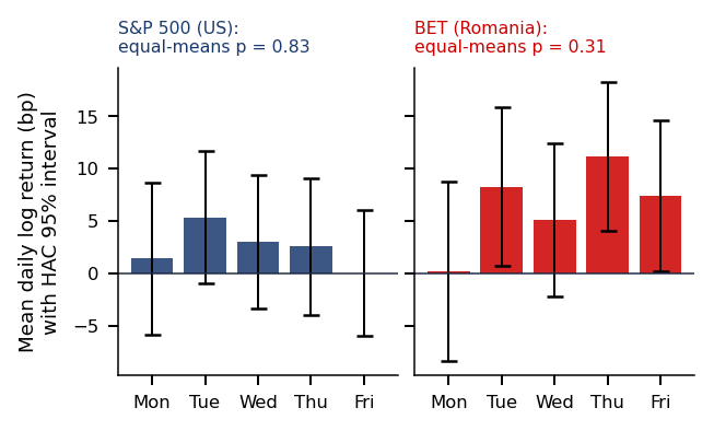
A calendar effect is a difference in mean returns associated with a day or a month. Three effects are tested in the chapter. The day-of-the-week effect is a difference in mean returns across Monday to Friday (French, 1980). The January effect is a difference between the mean January return and that of the other months (Rozeff & Kinney, 1976). The turn-of-the-month (TOM) effect concerns the last trading day of a month and the first three of the next (Ariel, 1987).
Each of these patterns was found by looking at data. Data snooping is the selection of a pattern after many alternatives have been searched on the same data; the selected pattern then looks significant even if no effect exists. The rest of the section quantifies this risk and corrects for it.
In brief
A calendar effect is a difference in mean returns associated with a day or a month.
Day-of-the-week effect: mean returns differ across Monday, Tuesday, …, Friday French (1980).
January effect: the mean January return differs from that of the other months Rozeff & Kinney (1976).
Turn-of-the-month (TOM) effect: higher mean returns on the last trading day of a month and the first three of the next Ariel (1987).
Data snooping: selecting a pattern after searching many alternatives on the same data.
How Many “Anomalies” Does Pure Chance Produce? (1/3)
A simulation is useful here because every null hypothesis in it is true, so every rejection is a false one. The experiment uses 2,000 trading rules with no economic content, applied to daily S&P 500 returns. Each rule picks 20% of the days at random and calls them "good days", and a \(t\) test compares the mean return on these days with the mean on the other days.
The chart shows the histogram of the 2,000 \(t\) statistics over the standard Normal density. Two pairs of vertical lines mark the thresholds \(|t| = 1.96\), the usual 5% level, and \(|t| = 3.0\), the stricter bar proposed by Harvey, Liu & Zhu (2016).
In brief
Why we simulate: here every null hypothesis is true, so every rejection is false.
Experiment: 2 000 trading rules with no economic content, on daily S&P 500 returns.
Each rule picks 20% of the days at random and calls them “good days”.
For each rule, a \(t\) test compares the mean return on “good days” with the mean on the other days.
The chart: the histogram of the 2 000 \(t\) statistics, over the standard Normal density.
The vertical lines: the thresholds \(|t| = 1.96\) (5%) and \(|t| = 3.0\), the bar proposed by Harvey, Liu & Zhu (2016).
How Many “Anomalies” Does Pure Chance Produce? (2/3)
In the interactive version, the first slider sets the number of rules tried, from 20 to 2,000, and the menu sets the share of "good days", from 5% to 50%. The ▶ button adds rules step by step, and "New rules" draws a new set of random rules.
Question for the room For 2,000 tests with valid p-values, which individual Bonferroni cutoff guarantees at most a 5% probability of any false rejection, regardless of dependence between tests?
Answer
The cutoff is 0.05/2,000 = 0.000025. The value 0.025 divides the level by two rather than by the number of tests; a two-sided p-value already includes both tails. The value 0.05 retains the individual level without controlling the family. Bonferroni's guarantee does not require independent tests. In the simulation, of 2,000 rules with no economic content, 104 (5.2%) have |t| > 1.96, six have |t| > 3.0, and the best has |t| = 3.30. Adding rules to the same family cannot lower the largest |t|.
The histogram follows the standard Normal density closely: under the null, the \(t\) statistics behave as the theory predicts. The rules beyond the vertical lines are those that a researcher who reports only the best result would call anomalies.
The result matches the test level: \(5.2\%\) of the random rules are "significant" at 5%, with \(|t| > 1.96\). The most spectacular rule has \(|t| = 3.30\), although it is pure chance; reported alone, it would pass even the strict bar \(|t| > 3.0\). That bar is passed by \(0.30\%\) of the random rules, 6 rules out of 2,000.
The lesson is that the number of rules tried, the family of tests, matters as much as the threshold chosen. A strict threshold reduces the share of false discoveries but does not remove them when the search is large enough. Sullivan, Timmermann & White (1999) show how to correct for data snooping in trading rules.
In brief
Result: \(5.2\%\) of the rules are “significant” at 5% (\(|t| > 1.96\)), as the test level implies.
The most “spectacular” rule has \(|t| = 3.30\), although it is pure chance.
reported alone, it would pass even the strict bar \(|t| > 3.0\).
The bar \(|t| > 3.0\) is passed by \(0.30\%\) of the random rules, i.e. 6 rules out of 2 000.
How many rules were tried (the family of tests) matters as much as the bar chosen.
The same logic applies to 15 real tests on daily data from 2000: five markets times three effects, the weekday, January and TOM effects. The markets compare two developed indices, the S&P 500 and the Euro Stoxx 50, with three emerging markets of the region, the BET (Romania), the WIG20 (Poland) and the BUX (Hungary).
The January extra return is the mean January return minus the mean of the other months, in percent per month. The TOM extra return is the mean return on TOM days minus the mean of the other days, in basis points per day (bp; 1 bp equals 0.01 percentage points).
The standard errors are heteroskedasticity and autocorrelation consistent (HAC), because returns show volatility clustering: HAC errors remain valid under it, while ordinary ones do not. In these tests the HAC errors are \(0.92\) to \(1.54\) times the ordinary ones, so the correction can make them smaller as well as larger.
In brief
HAC: Heteroskedasticity and Autocorrelation Consistent.
We apply the same logic to 15 real tests, on daily data from 2000.
five markets \(\times\) three effects (weekday, January, TOM).
We compare developed markets (S&P 500, Euro Stoxx 50) with emerging markets of the region (BET, WIG20, BUX).
January extra: the mean January return minus the mean of the other months, in percent per month.
TOM extra: the mean return on TOM days minus the mean of the other days.
in basis points per day (bp; 1 bp \(= 0.01\) percentage points).
We use HAC errors because returns show volatility clustering.
HAC errors remain valid under it; ordinary ones do not.
In these tests the HAC errors are \(0.92\)–\(1.54\) times the ordinary ones: smaller as well as larger.
The strongest results concern the turn of the month in the two smaller markets. The TOM extra return is \(+17.3\) bp per day for the BET and \(+15.1\) bp for the BUX, both with \(|t| > 3.5\), above the bar of \(3.0\) of Harvey, Liu & Zhu (2016). For the S&P 500 the TOM extra return is only \(+3.2\) bp per day, and we do not reject the null (\(t = 0.92\)).
The January effect is weaker. For the BET, January exceeds the other months by \(3.48\) percentage points, but the estimate is imprecise (\(t = 1.49\)). The BUX, with \(t = 2.25\), is the only market with a January-effect \(p\)-value below \(0.05\). For the day-of-the-week effect, we do not reject the null in any market; the smallest \(p\)-value is \(0.2265\), for the WIG20.
Fifteen tests were run, and the next frame asks which of them survive a correction for multiple testing. Even for the effects that survive, what the result supports is an association between the calendar and returns, not a mechanism.
In brief
Market
January extra (%/month)
\(t_{HAC}\)
TOM extra (bp/day)
\(t_{HAC}\)
S&P 500 (US)
\(-0.66\)
\(-0.80\)
\(3.2\)
\(0.92\)
BET (Romania)
\(3.48\)
\(1.49\)
\(17.3\)
\(3.62\)
Euro Stoxx 50
\(-0.30\)
\(-0.29\)
\(5.1\)
\(1.21\)
WIG20 (Poland)
\(0.53\)
\(0.40\)
\(8.2\)
\(1.72\)
BUX (Hungary)
\(2.66\)
\(2.25\)
\(15.1\)
\(3.63\)
TOM: the extra return is \(+17.3\) bp per day for the BET and \(+15.1\) bp for the BUX
The error rate controlled here is the family-wise error rate (FWER), the probability of at least one false rejection in the family of tests. It is the appropriate criterion when every anomaly reported should be real, not only most of them. With \(M\) independent tests at level \(\alpha\),
\[\text{FWER} = 1 - (1-\alpha)^M,\]
(2.11)
so for \(M = 15\) and \(\alpha = 5\%\) the FWER would be \(53.7\%\) if the tests were independent.
The Bonferroni procedure rejects a hypothesis only if \(p_i < \alpha/M\); it guarantees \(\text{FWER} \le \alpha\) under any dependence between the tests. The Holm procedure sorts the \(p\)-values, \(p_{(1)} \le \dots \le p_{(M)}\), and rejects step by step while
\[p_{(j)} < \frac{\alpha}{M - j + 1},\]
(2.12)
stopping at the first failure. Holm has the same guarantee as Bonferroni and rejects at least every hypothesis that Bonferroni rejects. Holm applied to the calendar tests is detailed in the Appendix, and bootstrap methods that exploit the correlation between tests, such as StepM, in a further appendix frame.
In brief
FWER: Family-Wise Error Rate — the probability of at least one false rejection in the family of tests.
Why FWER: we want every anomaly we report to be real, not only most of them.
With \(M\) independent tests at significance level \(\alpha\): \(\text{FWER} = 1 - (1 - \alpha)^M\).
For \(M = 15\) and \(\alpha = 5\%\), FWER would be \(53.7\%\) if the tests were independent.
Bonferroni: reject only if \(p_i < \alpha / M\).
it guarantees \(\text{FWER} \leq \alpha\) under any dependence between the tests.
Holm: sort \(p_{(1)} \leq \dots \leq p_{(M)}\) and reject while \(p_{(j)} < \alpha/(M - j + 1)\), stopping at the first failure.
Holm has the same guarantee and rejects at least everything Bonferroni rejects.
Bootstrap methods that use the correlation between tests (StepM): Appendix.
The three questions concern the meaning of a small \(p\)-value after a search over many rules, the meaning of a non-rejection, and the kind of new evidence that would confirm an anomaly.
In brief
Why does testing many rules change the meaning of a small p-value?
Does non-rejection prove efficiency?
Which new sample or robustness check would you request?
Searching over many rules creates more opportunities for a false rejection, so the same \(p\)-value is weaker evidence. A non-rejection does not prove efficiency: a test with low power may fail to reject even when the market is inefficient, and the conclusion concerns only the alternative tested, not every form of predictability.
The natural robustness check is the same rule on data after publication or on another market, where an artefact of data snooping disappears. A real effect usually weakens after publication but does not vanish (McLean & Pontiff, 2016).
In brief
Searching many rules creates more opportunities for false rejection.
No. A test with low power may fail to reject even if the market is inefficient.
The conclusion concerns only the alternative tested, not every form of predictability.
Example: the same rule on post-publication data or on another market.
a data-snooping artefact disappears out of sample.
A real effect usually weakens after publication but does not vanish McLean & Pontiff (2016).
The core of the chapter yields five results. The S&P 500 shows a reversal of returns at horizons of 2 to 10 days, with variance ratios below 1, while the BET shows persistence, with variance ratios above 1 at all four horizons tested. Out of sample, the dividend–price ratio does not beat the historical mean (\(R^2_{OS} < 0\)).
In the event study, the abnormal component of TLV's fall after the bank tax, measured against the BET, was almost offset over the next five sessions; a single event cannot separate an overreaction from later news. Among the calendar effects, only the TOM effects of the BET and the BUX remain significant after the Holm correction.
In brief
S&P 500: return reversal at horizons of 2–10 days (variance ratio below 1).
BET: persistence (variance ratio above 1) at all four tested horizons.
The dividend–price ratio does not beat the historical mean out of sample (\(R^2_{OS} < 0\)).
Bank tax: the abnormal component of TLV's fall, measured against the BET, was almost offset over the next five sessions.
a single event cannot separate overreaction from later news.
After the Holm correction only the TOM effects for the BET and the BUX remain significant.
Section summary
Pure chance makes \(5.2\%\) of 2,000 random rules significant at 5% and lets one of them reach \(|t| = 3.30\). The FWER of fifteen independent tests at 5% would be \(53.7\%\)(2.11), and the Holm procedure (2.12) keeps it below 5% under any dependence. On the fifteen calendar tests, only the turn-of-the-month effects of the BET and the BUX survive the correction; the January effect of the BUX (\(t = 2.25\)) does not.
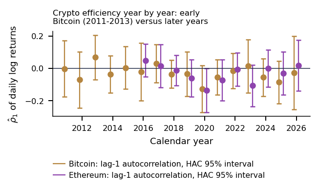
The chapter uses 16 daily series up to 18 September 2026; the sample sizes are in the Appendix. Thirteen are equity indices from 2000: four developed markets (S&P 500, Euro Stoxx 50, Nikkei 225, Hang Seng) and nine emerging or frontier markets (BET, WIG20, BUX, PX, BIST 100, Bovespa, IPC, Nifty 50, Shanghai). Bitcoin enters the full-sample and rolling tests from 2014, while the yearly crypto analysis starts in 2011. Ethereum starts in 2016, and the EUR/RON exchange rate, the reference rate of the National Bank of Romania (BNR), in July 2005.
Returns are daily log returns, \(r_t = \ln P_t - \ln P_{t-1}\), where \(P_t\) is the closing price, index level or exchange rate on day \(t\), each series on its own calendar. Equity indices use trading days only. A repeated close is removed only if the day shows no trading (zero volume, or open = high = low = close) or if its whole row copies the previous day's: such a day is a holiday filled with the previous price. A genuine unchanged close, with volume and an intraday range, stays as a zero return; the S&P 500 has 3 such days in about 6,700. The BET file has closes only, so none of its days is removed.
The IPC has 46 such days (44 of them in 2023–2026) with near-identical volume, likely duplicates from the data provider; they are kept, and dropping them moves \(\hat\rho_1\) by \(0.001\),\(z^*(2)\) by \(0.04\),\(\hat d\) by \(0.014\) and \(AQ\) by \(0.29\). Crypto-assets trade seven days a week, with 365 observations per year. Analyses that combine several series, such as event studies, align prices on common trading days before computing returns.
In brief
BNR: Banca Națională a României — the National Bank of Romania.
The standard answer to the question of what efficiency imposes on prices is the fair game: the return in excess of the required return cannot be forecast from the information set. The autocorrelation tests of the core check only one consequence of this condition. Because the required return comes from a pricing model, every test of the fair game is also a test of that model, the joint-hypothesis problem (Fama, 1991).
The condition leaves room for rational bubbles but rules out deviations from fundamental value that revert predictably, often called fads. Deviations do not always disappear, because arbitrage is risky when the convergence of prices is uncertain (Shleifer & Vishny, 1997); the limits of arbitrage are treated in Further Topics.
In brief
The question: what exact restriction does efficiency impose on prices, and what does it leave free?
The standard answer is the fair game.
The return in excess of the required return cannot be forecast.
The autocorrelation tests of section 2 check only one consequence of this condition.
The required return comes from a pricing model, so every fair-game test is also a test of that model Fama (1991).
A fair game allows rational bubbles.
but rules out deviations that revert predictably to fundamental value (fads).
An efficiency test is valid only under assumptions that the data may violate. The robust standard errors of autocorrelations, treated in Further Topics, require a finite fourth moment, \(\mathbb{E}[r^4] < \infty\). Heavy tails can break this condition: a Student \(t\) distribution with four degrees of freedom has a finite variance but an infinite fourth moment, and then the robust standard error no longer converges.
The critical values in use, \(\pm 1.96\) or the quantiles of the \(\chi^2\) distribution, are asymptotic approximations. They are correct as the sample grows but can be inaccurate in a short sample such as a window of 500 days. The limit theorems also need weak dependence, or mixing: observations far enough apart in time become nearly independent. Mixing allows volatility clustering and dependence between neighbouring days.
In brief
The question: which assumptions make an efficiency test valid, and which alternatives can it detect?
Robust standard errors of autocorrelations (Further Topics) need a finite fourth moment, \(\E[r^4]<\infty\)
heavy tails: Student \(t\) with four degrees of freedom has finite variance but \(\E[r^4]=\infty\), and then the robust standard error no longer converges
Critical values (\(\pm 1.96\), \(\chi^2\) quantiles) are asymptotic approximations
correct as the sample grows
possibly inaccurate in a short sample such as a 500-day window
Limit theorems also need weak dependence (mixing)
observations far enough apart in time become nearly independent
mixing allows volatility clustering and dependence between neighbouring days
A persistent predictor distorts inference in a finite sample. A predictor is predetermined when it is known before the return shock it is meant to predict; strict exogeneity also rules out correlation with the shocks at every other date. The dividend–price ratio of today can forecast the return of next month, but next month's price shock also changes the ratio, and this feedback rules out strict exogeneity.
Consistency is not the same as unbiasedness. With a merely predetermined predictor, the ordinary least squares (OLS) estimator converges to the true parameter as the sample grows, but it is biased in a finite sample.
In brief
Why does a persistent predictor distort inference in a finite sample?
A predetermined predictor is known before the return shock it predicts
strict exogeneity additionally rules out correlation with shocks at every date.
Today's dividend–price ratio can forecast next month's return.
yet next month's price shock also changes the ratio.
this feedback obstructs strict exogeneity.
Consistent is not unbiased.
with a merely predetermined predictor, OLS (Ordinary Least Squares) converges to the true parameter.
The question is whether dependence persists across horizons and market regimes. A process has short memory when its autocovariances are absolutely summable; an autoregressive model of order one, AR(1), with coefficient 0.5 has correlations \(0.5^k\) at lag \(k\). Long memory here means positive dependence that decays so slowly that the sum of the autocovariances diverges, which power-law decay can produce.
Scaling describes how a measure of fluctuations over \(n\) days, \(F(n)\), grows with the horizon, for example the standard deviation of a sum of \(n\) returns:
\[F(n) \propto n^H,\]
(2.13)
where \(H\) is the Hurst exponent, estimated in Further Topics. Doubling the horizon multiplies fluctuations by \(2^H\): by about 1.41 at \(H = 0.5\), without long memory, and by 1.68 at \(H = 0.75\). Anti-persistence describes increments that offset each other, as in fractional Gaussian noise (fGn) with \(H < 0.5\); fGn is a stationary Gaussian model of increments whose partial sums have variance proportional to \(n^{2H}\).
In brief
Does dependence persist across horizons and market regimes?
AR: AutoRegressive model.
Short memory has absolutely summable autocovariances
an AR(1) with coefficient 0.5 has correlations \(0.5^k\) at lag \(k\).
Long memory here means positive dependence decaying so slowly that the autocovariance sum diverges
power-law decay can produce this.
Scaling: a measure of fluctuations over \(n\) days, \(F(n)\), grows like \(n^H\)
e.g. the standard deviation of a sum of \(n\) returns
\(H\) is the Hurst exponent, estimated in Further Topics
doubling the horizon multiplies fluctuations by \(2^H\): about 1.41 at \(H = 0.5\) (no long memory) and 1.68 at \(H = 0.75\)
Anti-persistence describes offsetting increments, as in fractional Gaussian noise (fGn) with \(H<0.5\)
fGn is a stationary Gaussian increment model with partial-sum variance proportional to \(n^{2H}\).
For fGn the variance of a sum of \(q\) returns is \(\mathrm{Var}(r_t + \dots + r_{t-q+1}) = q^{2H}\,\mathrm{Var}(r_t)\), so the variance ratio (VR) is \(\mathrm{VR}(q) = q^{2H-1}\). Inverting the relation, an observed variance ratio implies a Hurst exponent
At \(q = 20\) days, the implied exponent is \(0.553\) for the BET and \(0.453\) for the S&P 500.
The difficulty is that a process without long memory can also give \(H(q) \neq 0.5\). An AR(1) with \(\rho_1 = -0.1\) has autocorrelations \(\rho_k = (-0.1)^k\), so only short memory, yet its \(\mathrm{VR}(20) = 0.826\) gives \(H(20) = 0.468\): the process looks anti-persistent without any long memory. At \(q = 250\) the same process gives \(H(250) = 0.482\); for short memory, \(H(q)\) approaches \(0.5\) as \(q\) grows.
An AR(1) with the BET's first-order autocorrelation, \(\hat\rho_1 = 0.109\), gives \(H(20) = 0.535\). Most of the gap between the BET's \(H(20) = 0.553\) and \(0.5\) is therefore short memory. Separating long from short memory requires a statistic built for the purpose, the modified rescaled-range (R/S) statistic of Lo (1991), treated in Further Topics.
In brief
For fGn, the variance of a sum of \(q\) returns is \(\Var(r_t + \dots + r_{t-q+1}) = q^{2H} \Var(r_t)\).
fGn: the exactly self-similar process defined above.
Hence \(\text{VR}(q) = q^{2H-1}\), and an observed \(\text{VR}(q)\) implies a Hurst exponent \(H(q) = 0.5 + \ln \text{VR}(q) / (2 \ln q)\).
At \(q = 20\) days, the implied exponent is \(0.553\) for the BET and \(0.453\) for the S&P 500.
The problem: a process without long memory can give \(H(q) \neq 0.5\)
Example: an AR(1) with \(\rho_1 = -0.1\) has autocorrelations \(\rho_k = (-0.1)^k\), so only short memory.
For this AR(1), \(\text{VR}(20) = 0.826\), so \(H(20) = 0.468\): the process looks “anti-persistent” without any long memory.
At \(q = 250\), the same process gives \(H(250) = 0.482\): for short memory, \(H(q)\) approaches \(0.5\) as \(q\) grows.
An AR(1) with BET's autocorrelation, \(\hat\rho_1 = 0.109\), gives \(H(20) = 0.535\).
So most of the gap between BET's \(H(20) = 0.553\) and \(0.5\) is short memory.
Separating long from short memory needs a statistic built for it: Lo's modified R/S (Further Topics).
The coefficients \(\hat a_i\) and \(\hat b_i\) are known exactly;
Firms are independent;
The variance of abnormal returns does not rise on the event day.
Each of them can fail.
Estimation error arises because \(\hat a_i\) and \(\hat b_i\) come from a finite window, so the predicted normal return is uncertain as well. Cross-sectional dependence arises because two banks hit by the same news have abnormal returns that move together. Event-induced variance arises because the event itself raises the variance, which the calm days of the estimation window understate. The corrections are given in the Appendix.
In brief
The question: how reliable are the \(t\) statistics of the Event studies section?
when their assumptions fail
There we assumed:
\(\hat a_i\) and \(\hat b_i\) are known exactly.
firms are independent.
the abnormal-return variance does not rise on the event day.
Estimation error: \(\hat a_i\) and \(\hat b_i\) come from a finite window.
the predicted normal return is also uncertain.
Cross-sectional dependence: two banks hit by the same news have abnormal returns that move together.
Event-induced variance: the event itself raises the variance.
The question is whether behavioural biases can explain the anomalies that survive correction. The frame begins with momentum, which comes in two forms. Cross-sectional momentum ranks assets against each other: if asset A gained 10% and asset B 2%, a relative strategy may buy A and sell B short. Time-series momentum uses the sign of each asset's own past return, so in the same example both A and B would receive positive signals. The behavioural explanations are in the Appendix.
In brief
Can behavioural biases explain the anomalies that survive?
Momentum
Cross-sectional momentum ranks assets.
if A gained 10% and B gained 2%, a relative strategy may buy A and short B.
Time-series momentum uses each asset's own past sign.
both A and B would receive positive signals in that example.
The question is what an in-sample rejection means when efficiency is tested with hundreds of predictors. Anomalies are found by searching among many predictors, and Harvey, Liu & Zhu (2016) count more than 300 published factors. The section on multiple testing showed that 2,000 random rules produce in-sample "anomalies". The Further Topics frames show how to evaluate a flexible model properly and why an in-sample rejection can arise even with rational investors (Martin & Nagel, 2022).
In brief
The question: what does an in-sample rejection mean?
when we test efficiency with hundreds of predictors
Anomalies are found by searching among many predictors: Harvey, Liu & Zhu (2016) count more than 300 published factors.
The case study tests a published result on weak-form efficiency in a market that did not exist when the classical tests were designed. Liu and Tsyvinski (2021) find that Bitcoin's weekly return predicts the returns of the following weeks. The course data reproduce the result in the authors' sample and test it on the eight years that followed.
The Question: Do Past Returns Predict Bitcoin's Return?
The question is whether this week's Bitcoin return predicts the returns of the following weeks. If it does, past prices contain information that the market has not used, a departure from weak-form efficiency. Liu and Tsyvinski (2021), in the Review of Financial Studies, find that cryptocurrency returns have no exposure to the usual stock-market or macroeconomic factors. They are predicted instead by factors specific to crypto markets: time-series momentum (TSMOM) and investor attention.
TSMOM means that a week with a high return is followed, on average, by high returns in the following weeks. In the authors' working paper of the National Bureau of Economic Research (NBER w24877), on Bitcoin from January 2011 to May 2018, the slope of the regression of next week's return on this week's return is 0.19 (\(t = 3.73\)). One more standard deviation of this week's return (16.6%) adds 3.2% to next week's return. The quintile of weeks with the highest returns is followed by 11.2% a week on average, the quintile with the lowest by 2.6%.
The result matters for efficiency because an effect that investors exploit should weaken after publication (McLean & Pontiff, 2016). The eight years after the authors' sample are a natural out-of-sample test.
In brief
Question: does this week's Bitcoin return predict the returns of the following weeks?
if so, past prices contain unused information: a departure from weak-form efficiency
The left panel shows the slope \(b_h\) of the predictive regression
\[R_{t+h} = a + b_h R_t + e_{t+h}, \qquad h = 1, \dots, 4 \text{ weeks},\]
(2.15)
with 95% intervals based on Newey–West (NW) standard errors, in the paper's sample and after it; the diamonds are the authors' numbers. The right panel shows the slope \(b_1\) over rolling windows of 104 weeks (two years), each dated at the last week of its window.
In the interactive version, the menu switches between Bitcoin and Ethereum, the first slider moves the end of the first period, and the second sets the length of the rolling window, from 52 to 208 weeks. The ▶ button moves the end of the first period through time.
Question for the room After May 2018, Bitcoin's slope is b₁ = 0.115, with NW t = 2.61. Which conclusion does this regression support?
Answer
The regression supports a one-week predictive association. A one-standard-deviation increase in the current return corresponds to an estimated 0.96-percentage-point increase in next week's return, compared with 2.98 percentage points in the earlier period. Neither a trading rule after costs nor out-of-sample forecast errors are evaluated. Using a sample after the paper's sample period does not replace that evaluation. Over rolling two-year windows, b₁ is significant in 13% of the windows.
In the paper's sample the course estimate of \(b_1\) lies close to the authors' diamond. After the sample, only the one-week slope stays away from zero, and the rolling panel shows how rarely a two-year window yields a significant slope. The numbers are on the result frame.
In brief
Left: the slope \(b_h\) in \(R_{t+h} = a + b_h R_t + e_{t+h}\), with 95% Newey–West (NW) intervals; diamonds: the authors' numbers
Right: the slope \(b_1\) over rolling windows of 104 weeks (two years), dated at the last week of the window
\(R_t\) is the simple return of Bitcoin in week \(t\), from one Sunday close to the next, computed from daily closing prices in Coordinated Universal Time (UTC), as in the paper. The predictive regression (2.15) is estimated for \(h = 1\) to 4 weeks in the paper's sample, 9 January 2011 to 27 May 2018 (386 weeks), and after it, 3 June 2018 to 13 September 2026 (433 weeks). The authors' robustness check, the same regression from 2013, is also reproduced. In the sort, the weeks are split into five quintiles by \(R_t\), and the mean of \(R_{t+1}\) is compared between the top and the bottom quintile.
The replication differs from the paper in three ways. The prices are those of the course data, from EODHD (EOD Historical Data), instead of CoinDesk prices. The standard errors are Newey–West with 5 lags instead of the authors' OLS and bootstrap standard errors. The attention factors (Google searches, Twitter) and Ripple are left out.
In brief
\(R_t\): the simple return of Bitcoin in week \(t\), from the Sunday close to the next Sunday close
daily closing prices in UTC (Coordinated Universal Time), as in the paper
Predictive regression \(R_{t+h} = a + b_h R_t + e_{t+h}\), for \(h = 1, \dots, 4\) weeks
the paper's sample: 9 Jan 2011 – 27 May 2018, 386 weeks
after the sample: 3 Jun 2018 – 13 Sep 2026, 433 weeks
the authors' robustness check: the same regression from 2013
Sorting: the weeks are split into five quintiles by \(R_t\); we compare the mean of \(R_{t+1}\) in the top and the bottom quintile
Differences from the paper
EODHD (EOD Historical Data) prices from the course data instead of CoinDesk prices
NW standard errors with 5 lags instead of the authors' OLS (ordinary least squares) and bootstrap standard errors
no attention factors (Google searches, Twitter) and no Ripple
The Result: Only the One-Week Effect Remains, Three Times Smaller
In the paper's sample, the course data reproduce the result: \(b_1 = 0.168\) (OLS \(t = 3.33\), NW \(t = 2.75\)), against 0.19 in the paper. The top quintile is followed by 9.9% a week and the bottom quintile by 2.6%, with a \(t\) statistic of 2.18 for the difference.
After the sample, predictability remains only at the one-week horizon. The slope is \(b_1 = 0.115\) (NW \(t = 2.61\)), and it survives the Holm correction over the four horizons (\(p = 0.009 < 0.05/4\)). At \(h = 2\), 3 and 4 the slopes lie between \(-0.026\) and \(0.072\), all with \(|t| \le 1.48\). One more standard deviation of this week's return adds 0.96% to next week's return, against 2.98% in the paper's sample, and weekly volatility fell from 17.7% to 8.3%. For Ethereum after the sample, \(b_1 = 0.107\) (NW \(t = 2.45\)).
What the result supports is statistical predictability of the one-week return, not a profitable strategy: the regression includes no trading costs, no risk adjustment and no out-of-sample forecasts. Three limits remain:
From 2013, within the paper's sample, \(b_1\) is no longer significant (NW \(t = 1.06\)), so the extreme weeks of 2011–2012 weigh heavily.
The slope is significant in only 13% of the rolling two-year windows.
The NW \(t\) test requires a finite fourth moment, which Chapter 1 questions.
In brief
In the paper's sample, the course data reproduce the result
\(b_1\) = 0.168 (OLS \(t\) = 3.33, NW \(t\) = 2.75), against 0.19 in the paper
the top quintile is followed by 9.9% a week, the bottom one by 2.6% (\(t\) of the difference = 2.18)
After the sample, predictability remains only at the one-week horizon
\(b_1\) = 0.115 (NW \(t\) = 2.61); it survives the Holm correction over the four horizons (\(p\) = 0.009 \(<\) 0.05/4)
at \(h\) = 2, 3, 4: slopes between \(-\)0.026 and 0.072, all with \(|t| \le\) 1.48
one more standard deviation today adds 0.96% to next week's return, against 2.98% in the paper's sample
weekly volatility fell from 17.7% to 8.3%; Ethereum after the sample: \(b_1\) = 0.107 (NW \(t\) = 2.45)
Type of evidence: statistical predictability of the one-week return, not a profitable strategy
no trading costs, no risk adjustment and no out-of-sample forecasts
Limits
from 2013, within the paper's sample, \(b_1\) is no longer significant (NW \(t\) = 1.06): the extreme weeks of 2011–2012 weigh heavily
\(b_1\) is significant in only 13% of the rolling two-year windows
the NW \(t\)-test requires a finite fourth moment, which Chapter 1 questions
Section summary
The course data reproduce the TSMOM slope of Liu and Tsyvinski in their sample (\(b_1 = 0.168\) against 0.19). After May 2018 only the one-week slope remains significant, \(b_1 = 0.115\), and the effect of one standard deviation falls from 2.98% to 0.96% a week. The result is predictability, not profit, and it depends on the extreme weeks of 2011–2012.
AI for scientific discovery
The last part of the core applies the chapter's tools to an open research question with the help of an artificial-intelligence (AI) assistant. The question is whether the entry of arbitrageurs through spot exchange-traded funds (ETFs) made Bitcoin more efficient. The frames show how a hypothesis proposed by the assistant is turned into a test with checks fixed before the results are seen.
An Open Question: Does a Market Become More Efficient When Arbitrageurs Enter?
The open question is whether Bitcoin's informational efficiency rises when new arbitrageurs enter through regulated instruments such as spot ETFs. Two strands of evidence bear on it. Tran & Leirvik (2020) find that the efficiency of crypto-assets varies over time and rises. Kia, Liu, Li, Song & Xu (2026) find that, after the launch of the spot ETFs, the spot market again became the dominant venue of price discovery.
Neither result says whether the change comes from the ETFs or from the maturing of the market. This is the question tested in the section; the ETF data and the placebo design are in the Appendix.
In brief
The question: does Bitcoin's informational efficiency rise when new arbitrageurs enter?
the new arbitrageurs come in through regulated instruments
such as spot ETFs
Tran & Leirvik (2020) find that the efficiency of crypto-assets varies over time and rises.
Kia, Liu, Li, Song & Xu (2026) find that, after the spot ETFs, the spot market again became the dominant venue of price discovery.
We do not know whether the change comes from the ETFs or from market maturity.
An AI assistant proposes a typical hypothesis: US spot Bitcoin ETFs, trading since 11 January 2024, brought arbitrageurs, so Bitcoin became more efficient. The discovery loop turns this claim into a test, with reusable prompts given in the Appendix. The literature step uses Kia, Liu, Li, Song & Xu (2026) and Tran & Leirvik (2020). The hypothesis is \(H_0: \rho_{1,\text{post}} = \rho_{1,\text{pre}}\), the equality of the first-order autocorrelation in two windows of equal length around the launch date, the first trading day. The data and code step uses the daily Bitcoin closing price in US dollars and first replicates the chapter's full-sample estimate, \(\hat\rho_1 = -0.022\).
The checks are fixed before any result is seen; the rationale for each is in the Appendix:
The standard errors of the estimates are HAC, not \(1/\sqrt{T}\);
The two windows have equal length;
The test uses the launch date only, plus placebo dates;
A control asset absorbs confounders such as the halving of April 2024, interest rates and fund inflows;
Every statistic tried enters a correction for multiple testing (Holm or Chow–Denning), and the minimum detectable effect (MDE) is reported.
The project asks whether the spot ETFs changed the time-varying efficiency of Bitcoin relative to a control asset. It uses the rolling variance ratio and detrended fluctuation analysis (DFA) of this chapter on Bitcoin and Ethereum; Ethereum serves as a control because it is untreated until July 2024. If parallel trends, no anticipation and no spillovers are not credible, the differences are reported as descriptive, not causal.
The first step is replication: the chapter's yearly Bitcoin autocorrelations and the numbers of the mini-case, recording which Bitcoin price series and which first date each window uses, placebo windows included. The hypotheses \(H_0\) and \(H_1\), the dates, the windows and the corrections are then pre-registered, committed before the results. The report contains robust inference, placebo tests and the MDE, and the code is published as a Quantlet. The prompts used are recorded in `AI_USE.md`, and every error of the AI assistant that was caught, such as an i.i.d. standard error or an invented reference, in `AI_ERRORS.md`.
In brief
Question: did the spot ETFs change the time-varying efficiency of Bitcoin?
relative to a control asset
rolling VR and DFA (this chapter) for Bitcoin and Ethereum; Ethereum is untreated until July 2024
if parallel trends, no anticipation and no spillovers are not credible, report descriptive, not causal, differences
Replicate first: the chapter's yearly Bitcoin autocorrelations and the mini-case numbers
record which Bitcoin price series and first date each window uses, placebo windows included
Pre-register: \(H_0\), \(H_1\), dates, windows and corrections, committed before the results
Report: robust inference, placebo tests and the MDE
Publish the code as a Quantlet
Log: record the prompts used in AI_USE.md
Record in AI_ERRORS.md every error of the AI assistant you caught
for example an i.i.d. standard error or an invented reference
Every efficiency claim in the chapter can be checked in five steps:
The information set \(\mathcal{I}_t\) that prices are assumed to reflect, past prices or public news.
The null hypothesis, RW1, RW3 or the martingale difference, stated together with the model of risk.
The statistic, with a variance that remains valid under volatility clustering.
The uncertainty created by the horizons, markets and windows tried, and the out-of-sample evidence.
The economic step: a statistical rejection is not an exploitable profit after costs, and a profit does not prove that the market is irrational.
The questions for self-checking ask why RW3 can be rejected for the S&P 500 while the market remains efficient in the economic sense, why the BET's \(H(20) > 0.5\) does not prove long memory, and which of two results, the BET's persistence or the non-rejection for Bitcoin, would survive a change of test, window and inference. Chapter 3 continues with risk-adjusted returns in factor models and the factor zoo. The reference textbooks are Campbell, Lo & MacKinlay (1997), chapter 2, and Franke, Härdle & Hafner (2019); advanced courses are listed in the Appendix.
In brief
Five steps for every efficiency claim
Information set: which information \(\mathcal{I}_t\) do we assume prices reflect (past prices, public news)?
Null: RW1, RW3 or the martingale difference (\(\E[r_t \mid \mathcal{I}_{t-1}] = \mu\), details in Further Topics), stated together with the risk model
Statistic: its variance valid under volatility clustering
Uncertainty: horizons, markets and windows tried, and out-of-sample evidence
Economics: a statistical rejection is not an exploitable profit after costs
a profit does not prove an irrational market
Check yourself and next steps
Why can RW3 be rejected for the S&P 500 while the market remains efficient in the economic sense?
Why does BET's \(H(20) > 0.5\) (the Hurst exponent implied by \(\text{VR}(20)\), Long memory) not prove long memory?
Which of the two results would survive a change of test, window and inference?
BET's persistence or Bitcoin's non-rejection
Next, Chapter 3: risk-adjusted returns with factor models
The decision has three parts: what I choose, under which conditions the choice holds, and what result would make me drop it.
For weak-form tests I choose robust standard errors, not i.i.d. ones: for the S&P 500, the robust standard error of \(\hat\rho_1\) is \(0.027\), against \(0.012\) under i.i.d. assumptions. Across the four variance-ratio horizons I use the Chow–Denning test, and across the 15 calendar tests the Holm correction. A predictor is judged by \(R^2_{OS}\) and the Clark–West test against the historical mean, not by the in-sample \(R^2\).
The choice holds under conditions. The robust standard errors require a finite fourth moment, which Chapter 1 questions. A rejection also tests the model of expected returns and is not a profit after costs.
Three results would make me drop a conclusion. For a predictor, \(R^2_{OS} < 0\) with an insignificant Clark–West test, as for \(dp\) on the S&P 500 (\(-0.51\%\),\(t = 0.42\)). For an anomaly, a rejection that does not survive Holm, as the January effect of the BUX (\(t = 2.25\)). For the BET's persistence, a variance ratio that stays inside the robust band on new windows.
In brief
What I choose
weak-form tests with robust standard errors, not i.i.d. ones (S&P 500: robust SE of \(\hat\rho_1\)\(0.027\), against \(0.012\))
Chow–Denning across the four variance-ratio horizons, Holm across the 15 calendar tests
for a predictor: \(R^2_{OS}\) and the Clark–West test against the historical mean, not the in-sample \(R^2\)
Under which conditions
the robust standard errors require a finite fourth moment, which Chapter 1 questions
a rejection also tests the model of expected returns and is not a profit after costs
What result would make me drop it
a predictor: \(R^2_{OS} < 0\) with an insignificant Clark–West test, as \(dp\) on the S&P 500 (\(-0.51\%\), \(t = 0.42\))
an anomaly: a rejection that does not survive Holm, as the BUX January effect (\(t = 2.25\))
the BET persistence: a variance ratio that stays inside the robust band on new windows
Section summary
Efficiency is a statement about an information set and a model of expected returns, and every test of it has to be read with a variance robust to volatility clustering, a correction for the family of tests tried and an out-of-sample check. On the chapter's data, the S&P 500 shows short-horizon reversal, the BET persistence that is mostly short memory, the dividend–price ratio fails out of sample, and only the turn-of-the-month effects of the BET and the BUX survive the Holm correction.
Further Topics
The frames in this part extend topics treated briefly in the body of the chapter, in the order in which the body refers to them. They give:
The numerical check behind the robust variance-ratio band, the case for the dividend–price ratio as a predictor and the Holm procedure on the calendar tests;
The theory of fair games, martingales, the risk-neutral measure and rational bubbles;
The construction of the autocorrelation, portmanteau, runs and variance-ratio tests with their robust versions;
HAC standard errors, the bootstrap and the Stambaugh bias of predictive regressions;
Long memory measured by R/S and detrended fluctuation analysis;
The Adaptive Markets Hypothesis and rolling measures of efficiency;
Event-study inference;
Calendar effects, time-series momentum and behavioural explanations;
Machine learning and rational learning with many predictors;
For a horizon of \(q = 2\) days the classical statistic is \(z = \sqrt{T}\,(\widehat{\text{VR}}(2) - 1)\), valid when returns are i.i.d. (RW1), while the robust statistic \(z^*\) divides the same numerator by \(\sqrt{\hat\theta(2)}\). Without volatility clustering \(\hat\theta(2) \approx 1\) and the two coincide; with clustering \(\hat\theta(2) > 1\) and \(|z^*| < |z|\). In a toy example with \(T = 400\) days and \(\widehat{\text{VR}}(2) = 0.90\),\(z = 20 \times (-0.10) = -2.0\) rejects at 5%, but \(\hat\theta(2) = 4\) gives \(z^* = -1.0\), which does not reject: the robust band around 1 is twice as wide. For the S&P 500, \(z = -8.15\) and \(z^* = -3.66\), about 2.2 times smaller, and the null is still rejected.
In brief
For \(q = 2\), the classical statistic is \(z = \sqrt{T}\,(\widehat{\text{VR}}(2) - 1)\).
it assumes i.i.d. returns (RW1).
The robust statistic \(z^*\) divides the same numerator by \(\sqrt{\hat\theta(2)}\).
Without volatility clustering, \(\hat\theta(2) \approx 1\) and \(z^* \approx z\).
with volatility clustering, \(\hat\theta(2) > 1\) and \(|z^*| < |z|\).
Toy example: \(T = 400\) days and \(\widehat{\text{VR}}(2) = 0.90\) give \(z = 20 \times (-0.10) = -2.0\): the null is rejected at 5%.
If volatility clustering makes \(\hat\theta(2) = 4\), then \(z^* = -2.0/\sqrt{4} = -1.0\) and the null is no longer rejected.
The robust band around 1 is then \(\sqrt{4} = 2\) times wider.
For the S&P 500, \(z = -8.15\) and \(z^* = -3.66\).
The Campbell–Shiller identity, \(dp_t \approx c + \sum_{j \ge 0} \rho^j (r_{t+1+j} - \Delta d_{t+1+j})\) with \(\rho\) just below 1 and \(\Delta d\) the log dividend growth, follows from the definition of the return through a log-linear approximation, without any economic model. If the log dividend–price ratio \(dp\) varies, it must therefore forecast future returns, future dividend growth or both. In the data \(dp\) forecasts dividend growth poorly, so its variation should forecast returns, which is why it is the most studied market predictor. A successful forecast would still not prove inefficiency, because it can reflect a risk premium that varies over time.
In brief
The Campbell & Shiller (1988) identity: \(dp_t \approx c + \sum_{j \ge 0} \rho^j \big(r_{t+1+j} - \Delta d_{t+1+j}\big)\).
\(\rho\) just below 1.
\(\Delta d\): log dividend growth.
The identity follows from the definition of the return through a log-linear approximation.
with no economic model.
Consequence: if \(dp\) varies, it must forecast future returns, future dividend growth or both.
In the data \(dp\) forecasts dividend growth poorly, so its variation should forecast returns Cochrane (2008).
The table collects the two-sided \(p\)-values of the calendar tests on five indices: the HAC \(t\) statistic against the Normal distribution for January and the turn of the month (TOM), and the Wald \(\chi^2_4\) test that the five weekday means are equal. The Holm procedure orders the 15 \(p\)-values and compares the \(k\)-th smallest with \(0.05/(16-k)\). The two smallest, TOM for the BET and TOM for the BUX, both 0.0003, lie below 0.0033 and 0.0036 and are rejected. The third, January for the BUX at 0.0245, exceeds 0.0038, so the procedure stops; without the correction it would have been a third rejection.
In brief
Two-sided \(p\)-values:
the HAC \(t\) statistic against the Normal distribution (January, TOM).
the Wald \(\chi^2_4\) test that the five daily means are equal (weekdays).
Market
Weekday, equal means
January
TOM
S&P 500 (US)
\(0.8263\)
\(0.4257\)
\(0.3585\)
BET (Romania)
\(0.3052\)
\(0.1368\)
\(0.0003\)
Euro Stoxx 50
\(0.6319\)
\(0.7738\)
\(0.2266\)
WIG20 (Poland)
\(0.2265\)
\(0.6865\)
\(0.0853\)
BUX (Hungary)
\(0.9327\)
\(0.0245\)
\(0.0003\)
The two smallest \(p\)-values are TOM for the BET and TOM for the BUX, both \(0.0003\).
They are below the Holm thresholds \(0.05/15 = 0.0033\) and \(0.05/14 = 0.0036\), so both nulls are rejected.
The third \(p\)-value, January for the BUX (\(0.0245\)), exceeds the threshold \(0.05/13 = 0.0038\), so Holm stops here.
Without correction, January for the BUX would have been the third rejection, since \(0.0245 < 0.05\).
The charts of the chapter label markets by short codes. US denotes the S&P 500 and HK Hong Kong; BIST, WIG20, BUX, PX and IPC are the benchmark indices of the Istanbul, Warsaw, Budapest, Prague and Mexican exchanges; BET is the benchmark index of the Bucharest Stock Exchange; FX denotes foreign-exchange series.
In brief
US: United States
HK: Hong Kong
BIST: Borsa İstanbul — the Istanbul Stock Exchange (BIST 100 index).
WIG20: Warszawski Indeks Giełdowy 20 — the Warsaw Stock Exchange index of the 20 largest companies.
BUX: Budapesti Értéktőzsde index — the Budapest Stock Exchange index.
PX: Prague Stock Exchange index (index Burzy cenných papírů Praha).
IPC: Índice de Precios y Cotizaciones — the Mexican Stock Exchange index.
A fair game for excess returns requires \(\mathbb{E}[r_{t+1} - \mu_t \mid \mathcal{I}_t] = 0\), where \(\mathcal{I}_t\) is the information available at the end of day \(t\) and \(\mu_t\) the required (equilibrium) return: the return beyond the compensation for risk cannot be forecast from \(\mathcal{I}_t\). A martingale is a process whose expected next value, given the past, equals its current value. With a constant required simple return \(m\), the value \(V_t\) of a position with dividends reinvested, discounted at \(m\),\(V_t/(1+m)^t\), is a martingale (Campbell, Lo & MacKinlay, 1997). Discounting at the risk-free rate gives a martingale only under the risk-neutral measure, and the price itself is a martingale only without dividends and with \(m = 0\).
In brief
Fair game for excess returns: \(\E[r_{t+1} - \mu_t \mid \mathcal{I}_t] = 0\)
\(\mathcal{I}_t\): the information available at the end of day \(t\); \(\E[\cdot \mid \mathcal{I}_t]\): the expectation given that information
\(\mu_t\): the required (equilibrium) return, the compensation for risk
in words: the return beyond \(\mu_t\) cannot be forecast from \(\mathcal{I}_t\)
Martingale: a process whose expected next value, given the past, equals its current value
with a constant required simple return \(m\), the value \(V_t\) of a position with dividends reinvested, discounted at \(m\), \(V_t/(1 + m)^t\), is a martingale Campbell, Lo & MacKinlay (1997)
discounting at the risk-free rate gives a martingale only under the risk-neutral measure (slide on the risk-neutral measure)
the price \(P_t\) itself is a martingale only if no dividends are paid and \(m = 0\); the expected log return is then negative (the Jensen term, next slide)
Because the logarithm is concave, the average of log outcomes is smaller than the log of their average unless the outcomes are constant. Equally likely simple returns of \(+10\%\) and \(-10\%\) have mean zero, but the mean log return is \(\tfrac12\ln(0.99) \approx -0.00503\). Along a path with one rise and one fall, wealth of 100 becomes \(100 \times 1.1 \times 0.9 = 99\): a zero arithmetic mean does not preserve compounded wealth.
In brief
The logarithm is concave.
averaging log outcomes gives less than taking the log of their average, unless outcomes are constant.
Equally likely simple returns of \(+10\%\) and \(-10\%\) have mean zero.
The mean log return is \(\tfrac12\ln(1.1)+\tfrac12\ln(0.9)=\tfrac12\ln(0.99)\approx-0.00503\).
Along a path with one rise and one fall, wealth 100 becomes \(100(1.1)(0.9)=99\).
a zero arithmetic mean does not preserve compounded wealth.
A martingale in prices, \(\mathbb{E}[P_{t+1} \mid \mathcal{I}_t] = P_t\), and a constant mean log return, \(\mathbb{E}[\ln(P_{t+1}/P_t) \mid \mathcal{I}_t] = \mu\), are different restrictions; they differ by the Jensen term, \(\mathbb{E}[\ln(1+R)] \approx \mathbb{E}[R] - \operatorname{Var}(R)/2\). The fair game implies that the unexpected return \(\varepsilon_{t+1} = r_{t+1} - \mu_t\) is uncorrelated with any function \(g(\mathcal{I}_t)\) of past information. With a constant \(\mu_t = \mu\), all autocorrelations \(\rho_k\),\(k \ge 1\), are zero, the hypothesis tested in the section on autocorrelation and variance ratios. The converse fails: zero autocorrelations do not rule out a mean that is nonlinearly predictable, which leads to the martingale difference hypothesis.
In brief
A martingale in prices and a constant mean log return are different restrictions
a martingale in prices: \(\E[P_{t+1} \mid \mathcal{I}_t] = P_t\)
a constant mean log return: \(\E[\ln(P_{t+1}/P_t) \mid \mathcal{I}_t] = \mu\)
the difference is the Jensen term: \(\E[\ln(1 + R)] \approx \E[R] - \Var(R)/2\), with \(R = P_{t+1}/P_t - 1\) the simple return
Consequence of the fair game: \(\text{corr}(\varepsilon_{t+1}, g(\mathcal{I}_t)) = 0\) for any function \(g\) of past information
where \(\varepsilon_{t+1} = r_{t+1} - \mu_t\) is the unexpected part of the return
If \(\mu_t = \mu\) is constant, all autocorrelations \(\rho_k = \text{corr}(r_t, r_{t-k})\), \(k \geq 1\), are zero
this is the hypothesis tested in section 2
The converse fails: zero autocorrelations do not rule out a nonlinearly predictable mean
the MDH (Martingale Difference Hypothesis), next topic
The martingale above uses the actual probabilities and the required return \(m\); pricing theory uses, equivalently, the risk-free rate and risk-adjusted probabilities. A risk-neutral measure is a set of pricing probabilities, in an arbitrage-free model, under which discounted traded prices, dividends included, are martingales. In the example a stock without dividends costs 100 today and will be worth 120 or 80 in one year, with a risk-free rate of 5%; the pricing probability \(q = 0.625\) gives \(0.625 \times 120 + 0.375 \times 80 = 105\), and \(105/1.05 = 100\). This \(q\) need not equal the actual probability of a rise: pricing probabilities are not forecasts of frequencies.
In brief
Why: the martingale above uses the actual probabilities and the required return \(m\).
pricing theory uses, equivalently, the risk-free rate and risk-adjusted probabilities.
A risk-neutral measure uses pricing probabilities, in an arbitrage-free model.
under which discounted traded prices, including dividends, are martingales.
Example: a stock without dividends costs 100 today.
in one year it is worth 120 or 80.
the risk-free rate is 5%.
The pricing probability \(q=0.625\) gives \(q\,120+(1-q)80=105\), and \(105/1.05 = 100\), today's price.
This \(q\) need not equal the actual probability of an increase.
pricing probabilities are not forecasts of frequencies.
The chart sets the two constructions of the previous frames side by side. On the left, under the actual probabilities, the conditional mean of the next value stays at 100; on the right, the pricing probabilities give an expected value of 105, whose value discounted at the risk-free rate is again today's price of 100.
In brief
Left: the actual conditional mean stays at 100. Right: pricing probabilities give 105, whose discounted value is 100.
With a constant required return \(m\), the fair game reads \(\mathbb{E}[P_{t+1} + D_{t+1} \mid \mathcal{I}_t] = (1+m) P_t\), where \(D_{t+1}\) is the dividend paid in \(t+1\). The fundamental value \(P^*_t = \mathbb{E}[\sum_{j \ge 1} D_{t+j}/(1+m)^j \mid \mathcal{I}_t]\) satisfies the same equation, so the pricing error \(B_t = P_t - P^*_t\) satisfies \(\mathbb{E}[B_{t+1} \mid \mathcal{I}_t] = (1+m) B_t\). The fair game ties the price to fundamental value only up to a rational bubble, a gap sustained by the expectation of resale and admissible only if it is expected to grow at the rate \(m\) (Chapter 17). A mean-reverting gap, a fad, makes \(\varepsilon_{t+1}\) predictable and violates the fair game, although short-horizon tests have little power against it (Summers, 1986). The restriction concerns the conditional mean only; volatility may be predictable (Chapter 1).
In brief
With a constant required simple return \(m\), the fair game is \(\E[P_{t+1} + D_{t+1} \mid \mathcal{I}_t] = (1 + m)\,P_t\)
\(D_{t+1}\): the cash flow (dividend) paid in \(t + 1\)
Fundamental value \(P^*_t = \E\big[\sum_{j \geq 1} D_{t+j}/(1 + m)^j \mid \mathcal{I}_t\big]\); pricing error \(B_t = P_t - P^*_t\)
The fundamental value \(P^*_t\) satisfies the same fair-game equation as the price
Subtracting the two equations, the gap \(B_t\) satisfies \(\E[B_{t+1} \mid \mathcal{I}_t] = (1 + m)\,B_t\)
A fair game ties the price to the fundamental value only up to a rational bubble
A gap \(B_t > 0\) sustained by the expectation of resale
A gap \(B_t \neq 0\) is admissible only if it is expected to grow at the required rate \(m\) (Chapter 17)
A mean-reverting gap (fad) makes \(\varepsilon_{t+1}\) predictable and violates the fair game, although short-horizon tests have little power against it Summers (1986)
A share pays 10 RON (Romanian leu) at the end of every year, forever, starting one year from today, and the required return is \(m = 10\%\), so the fundamental value is \(10/0.10 = 100\) RON. If the price today is 120 RON, the bubble is \(B_t = 20\) RON. Without a crash it grows to \(1.1 \times 20 = 22\) RON; after next year's dividend the fundamental value is still 100 RON and the price is 122 RON. The total simple return, \((122 + 10 - 120)/120\), is exactly the required 10%.
In brief
A share pays 10 RON (Romanian leu) at the end of every year, forever.
The first dividend is paid one year from today.
The constant required return is \(m=10\%\); fundamental value is \(P^*_t=10/0.10=100\) RON.
Today \(P_t=120\) RON, so \(B_t=20\) RON.
Without a crash, \(B_{t+1}=1.1\times20=22\) RON.
After next year's dividend, fundamental value remains 100 RON; the price is therefore 122 RON.
The total simple return is \((122+10-120)/120=10\%\).
Let the 20 RON bubble survive each year with probability \(\pi = 0.8\) and collapse to zero with probability 0.2, with both probabilities known to investors. The fair game for the bubble still requires an expected value of 22 RON, so conditional on survival the bubble must reach \(22/0.8 = 27.5\) RON, a conditional growth of 37.5%. The return is about 14.6% if the bubble survives (ex-dividend price 127.5 RON) and about \(-8.3\%\) if it bursts (price 100 RON); the expected return, \(0.8 \times 14.6\% + 0.2 \times (-8.3\%)\), is again 10%. The crash mechanism is that of Blanchard and Watson (1982): the expected return satisfies the fair game while either realised return can differ from it.
In brief
Initial bubble \(B_t=20\) RON and required return \(m=10\%\).
Survival probability \(\pi=0.8\); crash probability \(1-\pi=0.2\).
A crash makes the bubble zero; investors know the probabilities.
The fair game for the bubble, \(\E[B_{t+1}\mid\mathcal I_t]=(1+m)B_t\), requires an expected bubble of \((1+m)B_t=22\) RON.
Conditional on survival: \(B_{t+1}=22/0.8=27.5\) RON.
The fair game restricts only the expected return over the next period; it does not pin down the price level. The no-bubble (transversality) condition, \(\lim_{k\to\infty} \mathbb{E}[P_{t+k} \mid \mathcal{I}_t]/(1+m)^k = 0\), requires the discounted expected resale price to vanish as the resale horizon \(k\) grows, and under it the price equals the fundamental value, supported entirely by dividends. A rational bubble violates the condition: since \(\mathbb{E}[B_{t+k} \mid \mathcal{I}_t] = (1+m)^k B_t\), its discounted value stays \(B_t\) at every horizon, so the 20 RON bubble of the example is still worth 20 RON in today's money however distant the resale. Tirole (1985) shows that in overlapping-generations models a bubble can exist only if the interest rate is below the growth rate of the economy.
In brief
The fair game restricts only the expected return over the next period.
Gathering information costs analysts, data and computing. If prices reflected all information, nobody would be paid for collecting it, nobody would collect it, and prices could not reflect it (Grossman & Stiglitz, 1980). The resolution is an equilibrium degree of inefficiency, just large enough to reward informed traders for their costs. Large, liquid markets with cheap information and low costs should therefore be closer to efficiency, a prediction for the chapter's comparison of developed, emerging and crypto markets. Efficiency does not rule out bubbles either; it says that they are hard to time (Chapter 17).
In brief
Gathering information is costly (analysts, data, computing)
A pure arbitrage requires no positive initial outlay, cannot lose and gains in at least one state. Relative-value trading is different: it bets on the convergence of two prices, and convergence is uncertain. A price gap of 20 points may widen to 30 before it closes, and the position then needs extra collateral (margin) and may be liquidated. When convergence is uncertain, arbitrageurs with limited capital cannot eliminate deviations from fundamental value (Shleifer & Vishny, 1997), which is the link between arbitrage and efficiency.
In brief
Pure arbitrage is a strategy with:
no positive initial outlay.
no possible loss.
a positive gain in at least one state.
Relative-value trading is risky when price convergence is uncertain.
Example: a price gap of 20 points may widen to 30 before it closes.
the position then needs extra collateral (margin) and may be liquidated.
The link with efficiency: arbitrageurs with limited capital cannot eliminate deviations from fundamental value Shleifer & Vishny (1997).
The sample autocorrelation at lag \(k\) is \(\hat\rho_k = \sum_{t=k+1}^T e_t e_{t-k} / \sum_{t=1}^T e_t^2\), with \(e_t = r_t - \bar r\) the deviations of the \(T\) daily returns from their mean; \(\hat\rho_k > 0\) indicates persistence and \(\hat\rho_k < 0\) reversal. Under i.i.d. returns (RW1), \(\text{SE}(\hat\rho_k) \approx 1/\sqrt{T}\) and the 95% band is \(\pm 1.96/\sqrt{T}\). If the mean is unpredictable but volatility clusters (with finite fourth moments), the standard error under the null is \(\sqrt{\hat\tau_k}\):
When large moves cluster, \(\hat\tau_k\) in (2.16) exceeds \(1/T\), so the i.i.d. band is too narrow and classical tests reject too often. The robust statistics \(\tilde Q\) (Ljung–Box) and \(z^*\) (variance ratio) use \(\hat\tau_k\) instead of \(1/T\).
\(T\): number of daily returns; \(\bar r\): their mean; \(k\): the lag; \(\hat\rho_k > 0\): persistence, \(\hat\rho_k < 0\): reversal
Under RW1 (i.i.d.): \(\text{SE}(\hat\rho_k) \approx 1/\sqrt{T}\); 95% band \(\pm 1.96/\sqrt{T}\)
Unpredictable mean with volatility clustering (finite fourth moments): \(\text{SE}(\hat\rho_k) \approx \sqrt{\hat\tau_k}\)
\(\hat\tau_k = \sum_t e_t^2 e_{t-k}^2 \,/\, \big(\sum_t e_t^2\big)^2\) (robust variance under \(H_0\); for test bands centred at 0)
When large moves cluster, \(\hat\tau_k > 1/T\): the i.i.d. band is too narrow and classical tests reject too often; the robust statistics \(\tilde Q\) (Ljung–Box) and \(z^*\) (variance ratio) use \(\hat\tau_k\) instead of \(1/T\)
The standard error \(\sqrt{\hat\tau_k}\) is derived under the null, so it suits a test band centred at 0 but not an interval around an estimate \(\hat\rho_k \neq 0\). Around the estimate the chapter uses the heteroskedasticity- and autocorrelation-consistent (HAC) variance of the estimator (Newey & West, 1987): each day contributes \(\hat\psi_t = (e_t e_{t-k} - \hat\rho_k e_t^2)/\hat\gamma_0\) to \(\hat\rho_k - \rho_k\), and the variance of \(\hat\rho_k\) is the Bartlett-weighted long-run variance of \(\hat\psi_t\) divided by \(T\), with bandwidth \(\ell = \lfloor 4(T/100)^{2/9} \rfloor\): 9–10 lags for the full samples, 4–5 for one calendar year and 6 for the ETF windows. These intervals serve to compare periods, such as crypto years or the windows before and after the ETFs. A moving-block bootstrap gives similar values (S&P 500: HAC 0.030, block bootstrap 0.031, against \(\text{SE}_0 = 0.027\)), and the HAC standard error is smaller than \(\text{SE}_0\) for 14 of the 16 series (BET: 0.023 against 0.028).
In brief
\(\sqrt{\hat\tau_k}\) is derived under \(H_0\): valid for a test band centred at 0, not for an interval around \(\hat\rho_k \neq 0\).
Around the estimate we use the HAC variance of the estimator Newey & West (1987):
\(\hat\psi_t = (e_t e_{t-k} - \hat\rho_k e_t^2)/\hat\gamma_0\), with \(\hat\gamma_0 = \tfrac{1}{T}\sum_t e_t^2\): the contribution of day \(t\) to \(\hat\rho_k - \rho_k\).
\(\widehat{\Var}(\hat\rho_k) = \tfrac{1}{T}\big[\hat c_0 + 2\sum_{j=1}^{\ell}\big(1 - \tfrac{j}{\ell+1}\big)\hat c_j\big]\), with \(\hat c_j\) the lag-\(j\) autocovariance of \(\hat\psi_t\).
bandwidth \(\ell = \lfloor 4 (T/100)^{2/9} \rfloor\): 9–10 lags for the full samples, 4–5 for one calendar year, 6 for the ETF (Exchange-Traded Fund) windows.
Use: intervals around \(\hat\rho_k\) and comparisons between periods (crypto years, before/after the ETFs).
Check: a moving-block bootstrap (blocks of \(T^{1/3}\) days) gives similar values.
S&P 500: HAC \(0.030\), block bootstrap \(0.031\), \(\text{SE}_0 = 0.027\).
The HAC SE is smaller than \(\text{SE}_0\) for 14 of the 16 series (BET: \(0.023\) against \(0.028\)).
A portmanteau test combines several lag correlations into one statistic instead of selecting the most striking lag, and a Wald test does the same for restrictions on regression coefficients. Equal means on the five weekdays impose four restrictions, \(\beta_1 = \beta_2\),\(\beta_1 = \beta_3\),\(\beta_1 = \beta_4\),\(\beta_1 = \beta_5\), so the reference distribution is \(\chi^2_4\), with 5% critical value 9.49. Five restrictions, all \(\beta_d = 0\), would test a different null: that every weekday mean is zero.
In brief
A portmanteau test combines several lag correlations into one statistic.
instead of selecting the most striking lag.
A Wald test similarly tests coefficient restrictions jointly
five equal weekday means impose four restrictions, \(\beta_1=\beta_2\), \(\beta_1=\beta_3\), \(\beta_1=\beta_4\), \(\beta_1=\beta_5\), so the reference is \(\chi^2_4\), with 5% critical value 9.49.
Five restrictions, all \(\beta_d=0\), would test a different null: every weekday mean equal to zero.
both compared with \(\chi^2_m\). The robust limit holds under RW3 when the \(\hat\rho_k\) at different lags are asymptotically uncorrelated, as for a GARCH with symmetric innovations. At \(m = 10\) (critical value 18.31), the S&P 500 has \(Q = 97.1\) but \(\tilde Q = 20.0\)(\(p = 0.029\)), the BET \(Q = 108.0\) and \(\tilde Q = 24.4\)(\(p = 0.007\)), and Bitcoin \(Q = 20.2\)(\(p = 0.028\)) but \(\tilde Q = 11.9\)(\(p = 0.294\)). The robust test keeps the rejections for the S&P 500 and the BET but not for Bitcoin; \(\tilde Q\) requires a finite fourth moment, which Chapter 1 questions.
The runs test (Wald & Wolfowitz, 1940) uses only the signs of returns, with zero-return days dropped, so heavy tails do not affect it. A run is a maximal block of equal signs. With \(n_1\) positive and \(n_2\) negative days, \(n = n_1 + n_2\), independent signs give \(\mathbb{E}[R] = 2n_1 n_2/n + 1\) runs, and the standardised number of runs is approximately standard Normal, assuming a constant probability of a positive day. Too few runs (\(z < 0\)) mean persistent signs, too many (\(z > 0\)) alternating signs. The S&P 500 has \(z = 4.34\), alternation consistent with \(\hat\rho_1 < 0\); the BET has \(z = -6.05\), persistence consistent with \(\hat\rho_1 > 0\); Bitcoin has \(z = 2.68\), a rejection although \(\hat\rho_1\) is not significant: signs and magnitudes carry different information.
In brief
The runs test Wald & Wolfowitz (1940) uses only the signs of returns (zero-return days dropped), so heavy tails do not affect it
A run is a maximal block of equal signs: ++|-|+++ has 3 runs
With \(n_1\) positive days, \(n_2\) negative days and \(n = n_1 + n_2\), if the signs are independent:
Lo & MacKinlay (1988) estimate the variance ratio \(\text{VR}(q)\) from overlapping sums of \(q\) daily returns: \(\hat\sigma_a^2\) is the variance of one-day returns, \(\hat\sigma_c^2(q)\) the variance of the overlapping \(q\)-day sums divided by \(q\), with a divisor \(m = q(T-q+1)(1-q/T)\) that removes the small-sample bias, and \(\widehat{\text{VR}}(q) = \hat\sigma_c^2(q)/\hat\sigma_a^2\). Under RW1 (homoskedastic returns) the test statistic is
and \(|z| > 1.96\) rejects \(\text{VR}(q) = 1\) at 5%. The statistic (2.18) rejects too often under volatility clustering, which motivates the robust version.
In brief
Lo & MacKinlay (1988) estimate \(\text{VR}(q)\) from overlapping sums of \(q\) daily returns and correct the small-sample bias
\(\hat\mu\): mean daily return; \(\hat\sigma_a^2\): variance of one-day returns; \(\hat\sigma_c^2(q)\): variance of the overlapping \(q\)-day sums divided by \(q\); \(m\): a divisor that removes the small-sample bias
Test statistic under RW1 (homoskedastic returns, i.e. with constant variance)
Under RW3 plus the conditions of Lo & MacKinlay (1988) (finite moments, weak dependence and \(\mathbb{E}[\varepsilon_t^2 \varepsilon_{t-j}\varepsilon_{t-k}] = 0\) for \(j \neq k\)), the \(\hat\rho_k\) are asymptotically uncorrelated with variances \(\hat\delta_k/T\), where \(\hat\delta_k = T\hat\tau_k\) equals 1 without volatility clustering. Since \(\widehat{\text{VR}}(q) - 1\) weights \(\hat\rho_k\) by \(2(q-k)/q\), the robust statistic is
RW3 alone is not enough: the conditions hold for a GARCH with symmetric innovations but can fail with a leverage effect, in which case \(\hat\theta(q)\) needs the full covariance matrix of the \(\hat\rho_k\). At \(q = 5\) the S&P 500 has \(z^*(5) = -2.78\): the reversal stays significant with the robust standard error.
In brief
Under RW3 plus the conditions of Lo & MacKinlay (1988), the \(\hat\rho_k\) are asymptotically uncorrelated with variances \(\hat\delta_k / T\)
\(\hat\delta_k = T\hat\tau_k\), with \(\hat\tau_k\) of the autocorrelation slide: the robust variance of \(\sqrt{T}\hat\rho_k\), equal to 1 without volatility clustering
Asymptotic variance of \(\widehat{\text{VR}}(q)\) and the test statistic
\(2(q-k)/q\): the weight of \(\hat\rho_k\) in \(\widehat{\text{VR}}(q)\); \(|z^*| > 1.96\) rejects \(\text{VR}(q) = 1\) at 5%
RW3 alone is not enough
the conditions hold for GARCH with symmetric innovations
but can fail with a leverage effect
Without the condition \(\E[\varepsilon_t^2 \varepsilon_{t-j} \varepsilon_{t-k}] = 0\), \(\hat\theta(q)\) needs the full covariance matrix of the \(\hat\rho_k\)
At \(q = 5\), the S&P 500 has \(z^*(5) = -2.78\)
the reversal stays significant with the robust standard error
the comparison of \(z\) with \(z^*\) at \(q = 2\): section 2
The chart shows, for each of the 16 series of the chapter, the robust statistic \(z^*(5)\) of (2.19), with dashed lines at \(\pm 1.96\). Bars above the upper line indicate persistence over five days, bars below the lower line reversal.
At five days, \(|z^*(5)| > 1.96\) for the BET (2.98), the S&P 500 (\(-2.78\)), EUR/RON (2.19) and the Euro Stoxx 50 (\(-2.08\)). The joint test of Chow & Denning (1993), which takes the largest \(|z^*|\) over several horizons and compares it with the critical value 2.49, rejects RW3 for 5 of the 16 series: the BET, the S&P 500, EUR/RON, the IPC (at 2 days, \(z^* = 3.72\)) and Ethereum (at 20 days, \(z^* = 2.70\)). The Euro Stoxx 50 rejects at five days but not in the joint test, since its largest \(|z^*|\) is 2.24. The results give no ranking of the form "developed means efficient": the S&P 500 shows reversal, the BET and EUR/RON persistence.
In brief
Each bar on the previous chart is the robust statistic \(z^*(5)\) of one of the 16 series.
the dashed lines mark \(\pm 1.96\).
At 5 days, \(|z^*(5)| > 1.96\) for:
the BET (\(2.98\)), the S&P 500 (\(-2.78\)).
EUR/RON (\(2.19\)) and the Euro Stoxx 50 (\(-2.08\)).
The martingale difference hypothesis (MDH), \(\mathbb{E}[r_t \mid \mathcal{I}_{t-1}] = \mu\), states that no function of the past, linear or not, predicts the mean. RW3, which only sets all \(\rho_k\) to zero, is weaker. In the counterexample \(r_t = \varepsilon_t + \theta(\varepsilon_{t-1}^2 - \sigma^2)\), with \(\varepsilon_t\) i.i.d. symmetric and \(\sigma^2 = \operatorname{Var}(\varepsilon_t)\), all autocorrelations are zero, yet \(\mathbb{E}[r_t \mid \varepsilon_{t-1}] = \theta(\varepsilon_{t-1}^2 - \sigma^2)\) is predictable. The BDS test (Brock–Dechert–Scheinkman) (Brock, Dechert, Scheinkman & LeBaron, 1996) compares the frequency of nearby return sequences with that implied by i.i.d. observations; it tests i.i.d., not the MDH, and GARCH alone makes it reject, so a BDS rejection is evidence against RW1, not against weak-form efficiency.
In brief
MDH (Martingale Difference Hypothesis): \(\E[r_t \mid \mathcal{I}_{t-1}] = \mu\)
no function of the past predicts the mean, linear or not
\(\sigma^2 = \Var(\varepsilon_t)\), so the extra term has mean 0; \(\theta \neq 0\): how strongly yesterday's squared shock moves today's mean
all \(\rho_k = 0\), yet \(\E[r_t \mid \varepsilon_{t-1}] = \theta(\varepsilon_{t-1}^2 - \sigma^2)\) is predictable: autocorrelation tests cannot see it
The MDH tests on the next slide look for exactly this kind of dependence (results: Appendix)
The generalised spectral test (Escanciano & Velasco, 2006) measures the covariance between \(r_t\) and nonlinear functions \(e^{\mathrm{i}x r_{t-j}}\) of past returns at all lags \(j\), so it detects the counterexample of the previous frame, which autocorrelations miss. The automatic portmanteau test (Escanciano & Lobato, 2009) is a heteroskedasticity-robust Ljung–Box with the number of lags chosen from the data by a penalty; because it tests autocorrelations only, it does not detect the nonlinear counterexample.
In brief
Why: the counterexample on the previous slide shows that zero autocorrelations do not rule out a predictable mean
The generalised spectral test Escanciano & Velasco (2006) measures the covariance between \(r_t\) and nonlinear functions of past returns
\(e^{\mathrm{i}x r_{t-j}}\), at all lags \(j\)
it detects the counterexample \(r_t = \varepsilon_t + \theta(\varepsilon_{t-1}^2 - \sigma^2)\), which autocorrelations miss
In predictive regressions and on overlapping rolling windows the residuals are autocorrelated and heteroskedastic, and classical ordinary least squares (OLS) standard errors are not valid. In the dividend–price regression they are too small (OLS \(t = 1.16\), Newey–West \(t = 0.91\)), although HAC errors can also be smaller than OLS ones, as in the calendar-effects table. HAC standard errors estimate the long-run variance, the variance plus twice the sum of the autocovariances; Newey & West (1987) weight the autocovariance at lag \(j\) by \(1 - j/(\ell+1)\) so that the estimate is never negative. The bandwidth \(\ell\) is the number of lags included: with \(\ell = 5\) the weights of lags 1–5 are \(5/6, 4/6, \dots, 1/6\).
In brief
OLS: Ordinary Least Squares.
Why: the residuals are autocorrelated and heteroskedastic
in predictive regressions and on overlapping rolling windows
and classical OLS standard errors are then not valid
in the dividend–price regression they are too small (OLS \(t = 1.16\), Newey–West \(t = 0.91\))
HAC errors can also be smaller than OLS ones (the calendar-effects table)
HAC standard errors estimate the long-run variance
the variance plus twice the sum of the autocovariances
Newey & West (1987) weight the autocovariance at lag \(j\) by \(1 - j/(\ell + 1)\), so that the estimate is never negative
The bandwidth \(\ell\) is the number of lags included
with \(\ell = 5\) the weights of lags 1–5 are \(5/6, 4/6, \dots, 1/6\)
Neither the Stambaugh bias nor the DFA null band has a known exact distribution, and the bootstrap approximates it by generating many artificial samples under the null and recomputing the statistic in each. The i.i.d. bootstrap draws observations with replacement and destroys all dependence, volatility clustering included. The block bootstrap (Künsch, 1989) draws consecutive blocks and keeps the dependence within each block. The wild bootstrap multiplies each demeaned return by a random sign: it keeps each day's volatility but destroys serial correlation, reproducing an RW3-type null with symmetric signs, and is the one used for DFA.
In brief
Why: neither the Stambaugh bias nor the DFA null band has a known exact distribution
the bootstrap approximates it
The bootstrap generates many artificial samples under the null and recomputes the statistic in each
The i.i.d. bootstrap draws observations with replacement
and destroys all dependence, volatility clustering included
The block bootstrap Künsch (1989) draws consecutive blocks and keeps the dependence within each block
The wild bootstrap multiplies each demeaned return by a random sign
it keeps each day's volatility but destroys serial correlation: it reproduces an RW3-type null with symmetric signs (used for DFA)
The diagram compares the artificial samples of the bootstrap schemes of the previous frame. Blocks preserve the local ordering of returns, while sign flips preserve their absolute magnitudes; each scheme therefore imposes a different assumption on the artificial samples, and the choice determines which null hypothesis the resulting band represents.
In brief
Blocks preserve local ordering; sign flips preserve absolute magnitudes. They impose different assumptions on the artificial samples.
The question is why the dividend–price ratio of the section on out-of-sample predictability can look like a good predictor even when its true slope is zero. The model has two equations, \(r_{t+1} = \alpha + \beta x_t + u_{t+1}\) and \(x_{t+1} = \theta + \rho x_t + v_{t+1}\), with \(\operatorname{Cov}(u, v) = \sigma_{uv}\). Here \(r\) is the excess return, \(x\) the log dividend–price ratio \(dp_t = \ln D_t - \ln P_t\), with \(D_t\) the dividends of the last year, and \(\rho \approx 1\) its persistence, the AR(1) coefficient of \(dp\), distinct from the return autocorrelations \(\rho_k\) and from the \(\rho\) of the Campbell–Shiller identity.
In brief
Back to the regression of section 3: why can \(dp\) look like a good predictor even when \(\beta = 0\)?
\(D_t\): dividends paid over the last year; \(\beta\): the predictive slope, 0 if returns are unpredictable; \(\alpha\), \(\theta\): intercepts
\(\rho\): the persistence of \(x\), the AR(1) coefficient of \(dp\) (not the return autocorrelation \(\rho_k\), nor the \(\rho\) of the Campbell–Shiller identity); \(u\), \(v\): the shocks of the two equations; \(\sigma_{uv}\): their covariance; \(\sigma_v^2 = \Var(v)\); \(T\): number of periods
The predictor is predetermined but not strictly exogenous, so OLS is consistent but biased (Stambaugh, 1999). Projecting \(u\) on \(v\) gives \(\hat\beta - \beta = (\sigma_{uv}/\sigma_v^2)(\hat\rho - \rho)\) plus noise with mean zero, for instance when \((u, v)\) are i.i.d. with a bivariate Normal distribution. Since \(\hat\rho\) is biased downward in small samples (Kendall, 1954),\(\mathbb{E}[\hat\rho - \rho] \approx -(1+3\rho)/T\), the error passes into the slope:
A price rise lowers \(dp\), so \(\sigma_{uv} < 0\) and the bias in (2.20) is upward: predictability looks stronger than it is. Near a unit root the \(t\)-statistic is not standard Normal either, and valid inference uses the Bonferroni \(Q\)-test of Campbell & Yogo (2006).
In brief
\(x_t\) is predetermined, not strictly exogenous: OLS is consistent but biased Stambaugh (1999)
Project \(u\) on \(v\): \(u = (\sigma_{uv}/\sigma_v^2)\, v + e\), so \(\hat\beta - \beta = (\sigma_{uv}/\sigma_v^2)(\hat\rho - \rho) + \text{noise}\); \(e\): the part of \(u\) unrelated to \(v\)
Both regressions use the same months and the same \(x_t\), so the estimation errors \(\hat\beta - \beta\) and \(\hat\rho - \rho\) are linked through the correlation of the shocks \(u\) and \(v\); the noise term has mean zero when \(e\) is independent of the whole path of \(x\), e.g. \((u, v)\) i.i.d. with a bivariate Normal distribution
\(\hat\rho\) is biased downward in small samples Kendall (1954), and this error passes into \(\hat\beta\)
The inference of Campbell & Yogo (2006) allows for uncertainty about the persistence of the predictor instead of treating its estimate as known: it combines a confidence set for \(\rho\) with tests of the predictive slope over that set, allocating the error probability across the steps. For the S&P 500, \(\hat\rho = 0.9988\) and \(T(1-\hat\rho) = 1.4\), so a unit-root test cannot reject \(\rho = 1\), which is where the \(t\)-statistic of \(\hat\beta\) departs most from the standard Normal. This \(Q\)-test concerns predictive regressions and is not the Ljung–Box \(Q\) statistic.
In brief
Campbell–Yogo inference allows for uncertainty about predictor persistence. Campbell & Yogo (2006)
instead of treating its estimate as known.
It combines a confidence set for persistence with tests of the predictive slope over that set.
allocating the error probability across the steps.
For the S&P 500, \(\hat\rho = 0.9988\) and \(T(1 - \hat\rho) = 1.4\).
a unit-root test cannot reject \(\rho = 1\).
there the \(t\)-statistic of \(\hat\beta\) departs most from \(N(0,1)\).
This Q-test concerns predictive regressions
it is not the Ljung–Box Q statistic for autocorrelations.
The regression uses the monthly log excess return of the S&P 500 on the lagged \(dp_t\) over 1934–2026, \(T = 1\,111\) months. OLS gives \(\hat\beta = 0.267\) (percent per month per unit of \(dp\)) with Newey–West \(t = 0.91\), not significant even before any correction. With \(\hat\rho = 0.9988\),\(\operatorname{corr}(\hat u, \hat v) = -0.97\) and \(\hat\phi = \hat\sigma_{uv}/\hat\sigma_v^2 = -0.925\), formula (2.20) gives a bias of 0.333, so the corrected slope is \(0.267 - 0.333 = -0.066\): the estimated first-order correction exceeds the estimated slope. The correction is itself estimated, and Kendall's formula is least accurate when \(T(1-\hat\rho)\) is small, here 1.4, so \(-0.066\) indicates sign and size, not a precise slope. In a simulation with the same \(\rho\) and \(\operatorname{corr}(u, v)\),\(\beta = 0\) and 360 months, the nominal 5% \(t\)-test rejects in 26.5% of samples, more than five times too often.
In brief
Monthly log excess return regressed on the lagged \(dp_t\), 1934–2026, \(T = 1\,111\) months
OLS: \(\hat\beta = 0.267\), Newey–West \(t = 0.91\): not significant even before any correction
in % per month per unit of \(dp\)
Inputs: \(\hat\rho = 0.9988\), \(\text{corr}(\hat u, \hat v) = -0.97\), \(\hat\phi = \hat\sigma_{uv}/\hat\sigma_v^2 = -0.925\) (as fractions, not in %)
Substitution: bias \(= -100\,\hat\phi\,(1 + 3\hat\rho)/T = 0.333\) (in %, like \(\hat\beta\))
corrected slope \(= 0.267 - 0.333 = -0.066\): the estimated first-order bias correction exceeds the estimated slope
the correction is itself estimated: formal inference by Campbell & Yogo (2006) or a bootstrap
Kendall's formula is first order in \(1/T\) and least accurate when \(T(1 - \hat\rho)\) is small, here \(1.4\): read \(-0.066\) as indicative of the sign and size, not as a precise slope
Simulation: the nominal 5% \(t\)-test rejects \(\beta = 0\) in \(26.5\%\) of samples
with the same \(\rho\) and \(\text{corr}(u, v)\), \(\beta = 0\) and a 30-year sample (\(T = 360\) months)
The section on out-of-sample predictability defined the out-of-sample \(R^2_{OS}\) and applied the Clark–West test; this frame explains its form. Most published predictors have \(R^2_{OS} < 0\)(Welch & Goyal, 2008), which the update of Goyal, Welch & Zafirov (2024) confirms. The test of Diebold & Mariano (1995) compares the mean difference between the squared errors of two forecasts. The \(dp\) model nests the historical mean: under the null it estimates a zero \(\beta\), the noise of that estimate inflates its mean squared prediction error (MSPE), and the Diebold–Mariano test rejects less often than its nominal level. Clark & West (2007) add this noise back:
where \((\bar r_t - \hat r_t)^2\) is the part of the model's error due to estimating \(\beta\); the \(t\) test on the mean of \(f_t\) in (2.21) is one-sided, since only a positive gain is evidence for the predictor.
In brief
Section 3 defined \(R^2_{OS}\) and applied the Clark–West test to the S&P 500
The diagram contrasts short and long memory. The autocorrelations of an AR(1) process fade geometrically, while those of the fractional Gaussian noise (fGn) example fade slowly; the right panel compares how fluctuations grow with the horizon in the two cases, which is what the R/S and DFA statistics below measure.
In brief
AR(1) correlations fade geometrically; the fGn example fades slowly. The right panel compares fluctuation growth across horizons.
Using the rescaled range, Hurst (1951) found that years of high Nile floods followed other high-flood years more often than chance allows. For a window of \(n\) returns with mean \(\bar r_n\) and standard deviation \(s_n\), the cumulative deviations are \(Y_k = \sum_{i=1}^k (r_i - \bar r_n)\), the range is \(R_n = \max_k Y_k - \min_k Y_k\), and the statistic is \(R_n/s_n\). The scaling law
\[\mathbb{E}[R_n/s_n] \approx c\,n^H\]
(2.22)
defines the Hurst exponent \(H\) as the slope of \(\ln(R/S)\) on \(\ln n\), with \(R/S\) averaged over non-overlapping windows. \(H = 0.5\) means no long memory (short-run dependence is allowed), \(H > 0.5\) persistence with \(\rho_k \sim k^{2H-2}\), and \(H < 0.5\) anti-persistence.
In brief
Using the rescaled range, Hurst (1951) found that years of high Nile floods followed other high-flood years
The chart plots, for the S&P 500 and the BET, the average rescaled range \(R/S\) for each window length \(n\), together with the expectation for i.i.d. returns from the Normal distribution. The slope of \(\ln(R/S)\) on \(\ln n\) estimates the Hurst exponent of (2.22).
The solid line on the chart is the Anis & Lloyd (1976) expectation for i.i.d. returns from the Normal distribution. In small samples the raw slope exceeds 0.5 even for i.i.d. returns, and the Anis–Lloyd correction removes this bias: \(H_{AL}\) is 0.5 plus the slope of \(\ln(R/S) - \ln\mathbb{E}[R_n/s_n]\) on \(\ln n\). For the S&P 500 the raw exponent is 0.530 and the corrected one 0.485, so the apparent persistence came from small-sample bias. For the BET the raw exponent is 0.578 and the corrected one 0.533, so persistence remains. Whether this reflects long memory or only the lag-1 autocorrelation \(\hat\rho_1 = 0.109\) is an open question that the classical R/S statistic cannot settle.
In brief
On the previous chart, the dots show the average \(R/S\) for each window length \(n\).
The solid line is the Anis & Lloyd (1976) expectation for i.i.d. returns from the Normal distribution.
Lo (1991) shows that short-run autocorrelation inflates R/S and mimics long memory. His modification replaces \(s_n\) by a long-run (HAC) standard deviation \(\hat\sigma_\ell\), with \(\hat\sigma_\ell^2 = \hat\gamma_0 + 2\sum_{j=1}^\ell (1 - j/(\ell+1))\hat\gamma_j\), and uses the full sample: \(V = (\max_k Y_k - \min_k Y_k)/(\hat\sigma_\ell\sqrt{T})\), with bandwidth chosen as in Andrews (1991). Under short memory \(V\) lies in \([0.809, 1.862]\) with probability 95%. Short memory is not rejected for the S&P 500 (\(V = 1.560\)), Bitcoin (1.547), the PX (1.749) and EUR/RON (1.429); for the BET (\(V = 1.961\),\(\ell = 7\)) and Ethereum (1.980), \(V\) is just above the upper limit, weak evidence of long memory.
In brief
Lo (1991): short-run autocorrelation inflates R/S and mimics long memory
Modification: \(s_n\) is replaced by a long-run (HAC) standard deviation \(\hat\sigma_\ell\) with \(\ell\) lags
\(\hat\sigma_\ell^2 = \hat\gamma_0 + 2 \sum_{j=1}^{\ell} \big(1 - \tfrac{j}{\ell + 1}\big) \hat\gamma_j\) , \(\hat\gamma_j\): autocovariance at lag \(j\) (\(\hat\gamma_0\): the variance), with declining weights
\(V = \dfrac{\max_k Y_k - \min_k Y_k}{\hat\sigma_\ell \sqrt{T}}\) ; \(Y_k\): cumulative deviations over the full sample of \(T\) returns; bandwidth \(\ell\) chosen as in Andrews (1991)
Under short memory, \(V\) lies in \([0.809, 1.862]\) with probability \(95\%\)
\(V\) is inside the interval: short memory is not rejected
for the S&P 500 (\(V = 1.560\)), Bitcoin (\(1.547\)), PX (\(1.749\)) and EUR/RON (\(1.429\))
For the BET (\(V = 1.961\), with \(\ell = 7\) lags) and Ethereum (\(V = 1.980\)), \(V\) is just above \(1.862\)
Detrended fluctuation analysis (DFA) (Peng et al., 1994) measures how the fluctuation of cumulative returns grows with the window length. The profile \(y_k = \sum_{t \le k}(r_t - \bar r)\) is split into boxes of length \(n\); in each box a linear trend is fitted, and \(F(n)\) is the root mean square of all residuals, computed for many \(n\). Removing a linear trend from the profile removes a constant mean of returns in each box; if the mean itself trends, higher-order DFA is needed. The scaling \(F(n) \propto n^{\alpha_{DFA}}\) defines the exponent \(\alpha_{DFA}\), which plays the role of \(H\), with \(\alpha_{DFA} = 0.5\) meaning no long memory.
In brief
Peng et al. (1994): DFA measures how the fluctuation of cumulative returns grows with the window length.
Removing a linear trend from the profile removes a constant mean of returns in each box.
If the mean of returns itself trends, higher-order DFA is needed.
The algorithm
The profile \(y_k = \sum_{t \leq k} (r_t - \bar r)\) is the running sum of deviations from the mean, over the full sample.
The profile is split into boxes of length \(n\).
In each box a linear trend is fitted and the residuals are kept.
\(F(n)\) is the root mean square of all residuals; the calculation is repeated for many \(n\).
\(F(n) \propto n^{\alpha_{DFA}}\): the DFA exponent \(\alpha_{DFA}\) plays the role of \(H\) (\(\alpha_{DFA} = 0.5\): no long memory).
The null band for \(\alpha_{DFA}\) comes from a wild bootstrap with 199 replications, in which each residual \(e_t = r_t - \bar r\) is multiplied by a random sign \(\eta_t = \pm 1\) with probability 1/2. The sign flip keeps the volatility \(|e_t|\), allowed under RW3, and destroys only serial correlation, whereas a shuffle would destroy both. The implicit null is stricter than RW3, since it requires signs that are symmetric and independent given volatility, so the band is a benchmark, neither an exact test of RW3 nor a confidence interval for \(\alpha_{DFA}\).
In brief
The null band comes from a wild bootstrap (199 replications).
each residual \(e_t = r_t - \bar r\) is multiplied by a random sign \(\eta_t = \pm 1\), with probability \(1/2\).
The sign flip keeps the volatility \(|e_t|\), allowed under RW3, and destroys only serial correlation.
a shuffle would destroy both.
The implicit null is stricter than RW3: signs symmetric and independent, given volatility.
The band is therefore a benchmark, not an exact test of RW3 and not a confidence interval for \(\alpha_{DFA}\).
The chart shows the DFA exponent \(\alpha_{DFA}\) of each of the 16 series as a dot, with its 95% wild-bootstrap null band as a bar. A dot outside its own bar indicates memory that volatility clustering alone does not explain.
The S&P 500 (0.494), the Euro Stoxx 50 (0.488) and the Nikkei (0.503) are close to 0.5 and inside their bands. Three of the 16 series exceed the band: Ethereum (0.581), the BET (0.580, against an upper limit of 0.561) and, marginally, Bitcoin (0.576 against 0.575). The PX (0.553) and Shanghai (0.554) exceed only a band built by shuffling, which also destroys volatility clustering, so their apparent memory comes from volatility clustering. The local Whittle estimator (Robinson, 1995) estimates \(d = H - 0.5\) from the lowest frequencies; for the BET, \(\hat d = 0.118\) with 95% interval \([0.062, 0.174]\), but the interval assumes conditionally homoskedastic innovations, which volatility clustering violates. The evidence of long memory in returns is weak and depends on the method, while memory in volatility (Chapter 1) is strong.
In brief
Each dot on the previous chart is the exponent \(\alpha_{DFA}\) of one series.
the bar is the 95% wild-bootstrap null band.
S&P 500 (\(0.494\)), Euro Stoxx 50 (\(0.488\)) and Nikkei (\(0.503\)) are close to \(0.5\), inside the null band.
Three of the 16 series exceed the null band.
Ethereum (\(0.581\)).
BET (\(0.580\), against an upper limit of \(0.561\)).
and, marginally, Bitcoin (\(0.576\) against \(0.575\)).
PX (\(0.553\)) and Shanghai (\(0.554\)) exceed only a null band built by shuffling.
Shuffling also destroys volatility clustering.
their apparent memory comes from volatility clustering.
The local Whittle estimator Robinson (1995) estimates \(d = H - 0.5\) from the lowest frequencies.
for the BET, \(\hat d = 0.118\), 95% interval \([0.062, 0.174]\) (Appendix).
The interval assumes conditionally homoskedastic innovations.
volatility clustering violates this assumption.
so it is not decisive evidence.
Conclusion: the evidence of long memory in returns is weak and depends on the method.
Full-sample tests give weak and unstable evidence, and one possible reason is that efficiency varies over time. Andrew Lo proposed the Adaptive Markets Hypothesis (AMH) in Lo (2004) and developed it in the book Lo (2017). Markets are described as an ecology of competing species, traders, funds and algorithms, that adapt by trial and error rather than by perfect optimisation; efficiency is a matter of degree and depends on the number of competitors, the profit opportunities and the environment, and anomalies appear, weaken and may reappear. Time-varying statistics alone do not identify the AMH, because an Efficient Market Hypothesis (EMH) with time-varying risk premia also allows them.
Two strands of evidence support time variation. The survey of Lim & Brooks (2011) finds that stock-market efficiency varies over time, especially around crises. Urquhart & McGroarty (2016) find on four major indices (US, UK, Japan, euro area) that serial dependence appears and disappears across subperiods with market conditions.
In brief
Lim & Brooks (2011), a survey: stock-market efficiency varies over time, especially around crises
Urquhart & McGroarty (2016): serial dependence appears and disappears across subperiods with market conditions
Time-varying efficiency is measured by computing \(z^*(5)\) and the DFA exponent on rolling windows of 500 trading days, about two years, moved forward by 21 days, one month. The DFA band is computed by random sign flips, as before, but separately in each window, so that it follows the window's volatility. For comparison, a fixed band \([0.380, 0.615]\) is simulated from i.i.d. Student-\(t\) returns with 4 degrees of freedom: heavy tails without volatility clustering. Because clustering, allowed under RW3, raises \(\alpha_{DFA}\), the fixed band flags too many windows. Two cautions apply:
Overlapping windows are strongly correlated, so runs of rejections are not independent evidence;
About 5% of windows reject even under the null, so a share near 5% is a description, not a calibrated test of stability.
In brief
Compute a statistic on a rolling window
500 trading days (about two years)
moved forward by 21 days (one month)
Statistics: \(z^*(5)\) of the variance-ratio test and the DFA exponent
The DFA band is computed as before (random sign flips), but separately in each window
so it follows the window's volatility
For comparison, a fixed null band is \([0.380, 0.615]\)
simulated from i.i.d. Student-\(t\) returns with 4 degrees of freedom
heavy tails, no volatility clustering
The fixed band ignores volatility clustering, allowed under RW3
volatility clustering raises \(\alpha_{DFA}\)
so the fixed band flags too many windows
Two cautions for reading the results
Overlapping windows are strongly correlated: runs of rejections are not independent evidence
Even under the null about 5% of windows reject; a share near 5% is a description, not a calibrated test of stability
The chart plots \(z^*(5)\) on rolling 500-day windows, dated by their last day, with dashed lines at \(\pm 1.96\). The share of windows with \(|z^*(5)| > 1.96\) is 6.7% for the S&P 500, 22.4% for the BET and 0.0% for Bitcoin. The S&P 500 is negative in almost every window but beyond \(-1.96\) only in windows ending in 2008–2010. The BET rejects in episodes, in windows ending in 2002–2005, 2013–2014, 2018 and after 2023. The FTSE (Financial Times Stock Exchange, FTSE Russell, index provider) upgrade of Romania on 21 September 2020 shows no break: the BET statistic was near zero from 2016 and rises again after 2023.
In brief
\(z^*(5)\) on rolling 500-day windows, dated by the last day
dashed lines \(\pm 1.96\)
Share of windows with \(|z^*(5)| > 1.96\): S&P 500 \(6.7\%\), BET \(22.4\%\), Bitcoin \(0.0\%\)
S&P 500: negative in almost every window, beyond \(-1.96\) only in windows ending in 2008–2010
BET: episodes (windows ending in 2002–2005, 2013–2014, 2018 and after 2023)
The upgrade by the index provider FTSE Russell (FTSE: Financial Times Stock Exchange) of 21 Sep 2020 (Appendix) shows no break
BET was near zero from 2016 and rises again after 2023
The chart plots \(\alpha_{DFA}\) on rolling 500-day windows for the S&P 500, the BET and Bitcoin, with the 95% wild-bootstrap null band of each window shaded around it.
Outside their own band are 1.7% of the windows for the S&P 500, 3.1% for the BET and 0.0% for Bitcoin; with the fixed Student-\(t_4\) band the shares are 6.7%, 11.2% and 1.1%. The fixed band ignores volatility clustering, and the extra DFA exceedances of the BET came from it. The BET episodes of the variance-ratio chart remain, because they concern autocorrelation over a few days, short memory, which the DFA exponent does not target. Power is low: the BET band averages \([0.36, 0.64]\), and 500 observations cannot pin down a scaling exponent.
In brief
\(\alpha_{DFA}\) on rolling 500-day windows.
shaded: the wild-bootstrap 95% null band computed in each window.
Outside their own band: S&P 500 \(1.7\%\), BET \(3.1\%\), Bitcoin \(0.0\%\) of windows.
With a fixed Student-\(t_4\) band: \(6.7\%\), \(11.2\%\), \(1.1\%\).
the fixed band ignores volatility clustering.
the extra DFA exceedances of the BET came from volatility clustering.
The BET episodes in the variance-ratio chart remain.
they concern autocorrelation over a few days (short memory).
the DFA exponent does not target short memory.
Low power: the BET band averages \([0.36, 0.64]\).
500 observations cannot pin down a scaling exponent.
Kim, Shamsuddin & Lim (2011) show, over a century of US data, that predictability varies with market conditions such as crises and bubbles rather than along a declining trend, and make the AMH testable by linking it to state variables. The chapter's version regresses the rolling \(z^*(5)\) on the window's annualised volatility (in percent) and a crisis indicator equal to 1 if the window overlaps September 2008–June 2009 or February–June 2020, with Newey–West errors of 24 lags because consecutive windows share 95% of their days. For the S&P 500 the crisis coefficient is \(-0.71\)(\(t = -2.53\)) and the volatility coefficient 0.008 (\(t = 0.39\)),\(R^2 = 0.21\); for the BET they are \(-0.82\)(\(t = -2.77\)) and \(-0.008\)(\(t = -0.36\)),\(R^2 = 0.15\). In crisis windows \(z^*(5)\) is lower, closer to reversal, even at equal volatility. The result supports an association conditional on volatility, not a causal effect; it is consistent with the AMH but does not identify it, because a change in \(z^*(5)\) can come from \(\widehat{\text{VR}}(5) - 1\) or from its standard error.
The AMH predicts that a new market becomes more efficient over time: \(\hat\rho_1 \neq 0\) in Bitcoin's early years and values near zero later. The chart shows \(\hat\rho_1\) of daily returns in each calendar year, with the HAC 95% interval, for Bitcoin and Ethereum. For Bitcoin in 2011–2013 the intervals are wide and include zero, so the data do not show the early inefficiency the AMH predicts.
In brief
The AMH predicts that a new market becomes more efficient over time
\(\hat\rho_1 \neq 0\) in Bitcoin's early years, values near zero later
The chart: \(\hat\rho_1\) of daily returns in each calendar year, with the HAC 95% interval, for comparing years
Bitcoin 2011–2013: the intervals are wide and include zero
the data do not show the early inefficiency the AMH predicts
Only one of the 27 yearly autocorrelations, 16 for Bitcoin and 11 for Ethereum, is significant at 5%: Ethereum in 2023, \(\hat\rho_1 = -0.107\), against about 1.35 expected by chance alone. The test uses \(\text{SE}_0\), derived under the null, while the chart's bars use the HAC standard error, which is why the bar of Ethereum 2020 excludes 0 and that of 2023 does not. Urquhart (2016) rejects efficiency in the early years with other tests, another price source and classical standard errors. Power is limited: one year of 365 returns gives a robust standard error of about 0.05–0.13, so small effects are invisible, and the robust error itself requires a finite fourth moment, which Chapter 1 questions.
In brief
Only one of the 27 yearly autocorrelations is significant at 5%: Ethereum in 2023, \(\hat\rho_1 = -0.107\)
16 for Bitcoin, 11 for Ethereum
by chance alone we would expect about \(1.35\)
the test uses \(\text{SE}_0\) (derived under \(H_0\)), the chart's bars the HAC SE: the bar of Ethereum 2020 excludes 0, that of 2023 does not
where \(T_0\) is the number of estimation days, \(\sigma_\varepsilon^2\) the residual variance, \(r_{m,\tau}\) the market return on the event day and \(\hat\mu_m\),\(\hat\sigma_m^2\) the mean and variance of the market return in the estimation window. The bracket in (2.23) grows when the event-day market move is unusual: for the bank tax of the section on event studies, the extreme BET move makes it 2.12, hence \(t = -6.85\) instead of \(-10.0\) for TLV, and \(t = -4.03\) for BRD. Boehmer, Musumeci & Poulsen (1991) standardise each abnormal return by its own prediction error and estimate the variance from the firms' standardised values on the event day, so the test stays valid if the event raises the variance.
When all \(N\) firms have the event on the same day, their abnormal returns are correlated, with average correlation \(\bar\varrho\) estimated in the estimation window; for TLV and BRD, \(\bar\varrho = 0.153\). A test that assumes independence ignores the covariances, and the true variance of the mean is \(1 + (N-1)\bar\varrho\) times larger. For TLV and BRD the independence-based \(t\) of \(-7.55\), divided by \(\sqrt{1 + \bar\varrho} = 1.074\), becomes \(-7.03\), the \(t\) of the equal-weighted portfolio, which allows for the correlation automatically. A cross-sectional variance estimate, as in Boehmer, Musumeci & Poulsen (1991), further understates the variance by the factor \(1 - \bar\varrho\), which is why Kolari & Pynnönen (2010) multiply the statistic by \(\sqrt{(1-\bar\varrho)/(1+(N-1)\bar\varrho)}\). With ten firms and the same correlation, the understatement is a factor of 2.38 for the independence-based test and 2.81 for the cross-sectional one.
In brief
The question: what happens to the test of \(\overline{AR}_0\) when all firms have the event on the same day?
Let \(N\) be the number of firms and \(\bar\varrho\) the average correlation of their abnormal returns.
estimated in the estimation window.
for TLV and BRD, \(\bar\varrho = 0.153\).
The test that assumes independence ignores the covariances.
with \(\bar\varrho > 0\) the true variance of the mean is \(1 + (N-1)\bar\varrho\) times larger.
For TLV and BRD, the \(t\) computed under independence is \(-7.55\).
divided by \(\sqrt{1 + \bar\varrho} = 1.074\) it becomes \(-7.03\).
That is the \(t\) of the equal-weighted portfolio, which allows for the correlation automatically.
An anomaly is a return pattern that the asset-pricing model does not explain, and it has three possible explanations: an omitted risk factor, mispricing due to a behavioural bias, or data snooping. Anomalies come in families:
Time-series effects, such as time-series momentum;
Cross-sectional effects, such as size, value and momentum (Chapter 3).
Returns on published anomalies fall by 26% after the end of the sample studied and by 58% after publication (McLean & Pontiff, 2016). The day-of-week effect is estimated from \(r_t = \sum_{d=1}^5 \beta_d D_{d,t} + u_t\), where \(D_{d,t}\) marks weekday \(d\) and \(\beta_d\) is its mean return; the Wald test of \(\beta_1 = \dots = \beta_5\)(\(\chi^2_4\)) uses HAC errors (Newey & West, 1987) with 5 lags, because \(u_t\) is heteroskedastic and autocorrelated.
In brief
The question: which patterns survive the correction for multiple testing, and what explains them?
An anomaly is a return pattern the asset-pricing model does not explain.
The chart shows the mean daily log return by weekday over 2000–2026, in basis points (bp, 1 bp = 0.01%), with HAC 95% intervals. For the S&P 500 there is no Monday effect since 2000, unlike in French (1980): the means range from 0.0 bp on Friday to 5.3 bp on Tuesday, and the test of equal means has \(p = 0.83\). For the BET, Thursday has 11.2 bp (\(t = 3.09\)), yet the joint test gives \(p = 0.31\). The two results answer different nulls: that a day's mean is zero, which mixes the day effect with the positive average return, and that all five means are equal, which is the day effect itself.
In brief
Mean daily log return by weekday, in basis points (bp), 2000–2026, HAC 95% intervals
1 bp = 0.01%
S&P 500: we find no Monday effect since 2000, unlike French (1980)
from \(0.0\) bp (Friday) to \(5.3\) bp (Tuesday)
equal-means \(p = 0.83\)
BET: Thursday \(11.2\) bp (\(t = 3.09\)), yet the joint test gives \(p = 0.31\)
Two different nulls:
a day's mean equal to zero (mixes the day effect with the positive average return)
Time-series momentum (TSMOM) (Moskowitz, Ooi & Pedersen, 2012) goes long an index when the sum of its past 12 monthly log returns is a gain and short otherwise: the signal is \(s_t = \text{sign}(\sum_{j=1}^{12} r_{t-j})\) and the strategy return is \(s_t R_t\), with \(R_t\) the index return of month \(t\). On the next chart, each bar is the HAC \(t\) statistic (6 lags) of the strategy's mean monthly return in one market.
The chart shows, for each of the 15 markets, the HAC \(t\) statistic of the mean monthly TSMOM return. Bars beyond 1.96 are significant at 5% when each market is taken alone, before any correction for multiple testing.
Taken alone, the strategy has a mean return significant at 5% for the BET (1.40% a month, \(t = 2.68\)) and the S&P 500 (\(t = 2.22\)), while Bitcoin has \(t = 1.94\). With 15 markets tested, the first Holm threshold is \(0.05/15 = 0.0033\), and the smallest \(p\)-value, that of the BET, is 0.007, so no market remains significant after the correction. The annualised TSMOM Sharpe ratio, computed on price indices without dividends or a risk-free rate, is below buy-and-hold: 0.65 against 0.75 for the BET and 0.48 against 0.52 for the S&P 500. Part of the TSMOM return may be the equity premium earned in the months spent long. The result supports a comparison of procedures.
In brief
Taken alone, the strategy has a mean return significant at 5%:
for the BET (\(1.40\%\) a month, \(t = 2.68\)).
the S&P 500 (\(t = 2.22\)).
For Bitcoin, \(t = 1.94\), below \(1.96\).
But we tested 15 markets.
the first Holm threshold is \(0.05/15 = 0.0033\).
the smallest p-value, the BET's, is \(0.007\).
After the multiple-testing correction, no market remains significant.
The TSMOM Sharpe ratio is below buy-and-hold: \(0.65\) vs \(0.75\) for the BET, \(0.48\) vs \(0.52\) for the S&P 500.
Type of evidence: comparison of procedures.
Part of the TSMOM return may be the equity premium, earned in the months spent long.
the mean stock return over the risk-free rate.
The Sharpe ratio is annualised (full table: Appendix).
\(\sqrt{12}\times\) monthly mean over monthly SD.
on price indices without dividends or a risk-free rate.
The behavioural explanations of anomalies rest on a few concepts:
In prospect theory gains and losses are judged relative to a reference point, losses weigh more than equal gains (loss aversion) and small probabilities are overweighted.
The disposition effect is the tendency to sell winners and keep losers.
Anchoring is excess weight on an initial number, such as the purchase price.
Overconfidence overstates the precision of one's beliefs and leads to too much trading.
Limited attention leaves relevant information unprocessed.
Herding follows others' actions without an independent assessment.
Underreaction and overreaction describe a price that adjusts too little or too much to news at first, the second followed by reversal.
In brief
Prospect theory: gains and losses are judged relative to a reference point.
losses weigh more than equal gains (loss aversion).
small probabilities are overweighted.
Disposition effect: the tendency to sell winners and keep losers.
Anchoring: excess weight on an initial number, such as the purchase price.
Overconfidence: overstating the precision of one's beliefs, which leads to too much trading.
Limited attention: relevant information left unprocessed.
Herding: following others' actions without an independent assessment.
Underreaction and overreaction: a price adjusts too little or too much to news at first.
Shiller (1981) documents excess volatility: prices move far more than the dividends that should justify them. De Bondt & Thaler (1985) use overreaction to explain return reversals over 3–5 years, and prospect theory (Kahneman & Tversky, 1979) explains the disposition effect. In an illiquid market such as the Bucharest Stock Exchange, herding produces log-periodic bubbles, with prices rising super-exponentially and ever faster oscillations before the crash (Pele, Mazurencu-Marinescu & Nijkamp, 2013); today its channels are order books, algorithms and social media (Chapter 10). Biases alone do not break efficiency, because rational arbitrageurs could trade against them; the next frame asks whether they can.
Real arbitrage is risky and needs capital (Shleifer & Vishny, 1997). Noise-trader risk means that mispricing can get worse before it corrects (De Long, Shleifer, Summers & Waldmann, 1990), where noise traders trade on signals without information content, such as sentiment or rumours. Funding constraints force managers who lose clients after losses to close positions at the worst time, and short-selling limits, margins, trading costs and the lack of perfect substitutes add costs. Anomalies can therefore persist where arbitrage is hard: in the small, illiquid Romanian market the BET shows the strongest persistence among the stock indices. The AMH reconciles both views, with rational and biased behaviour coexisting and evolving.
Machine learning (ML) learns a prediction rule from data (Chapter 13) and can capture nonlinear patterns that autocorrelation tests miss. In the US cross-section, Gu, Kelly & Xiu (2020) find that trees and neural networks give large economic gains over linear regressions, although their monthly out-of-sample \(R^2\) is below 1%. Large language models read news and filings, and Tak & Pele (2025) forecast stock trends with LLaMA.
In brief
ML (machine learning) learns a prediction rule from data (Chapter 13)
captures nonlinear patterns that autocorrelation tests miss
Gu, Kelly & Xiu (2020): trees and neural networks give large economic gains over linear regressions
in the US cross-section
yet their monthly out-of-sample \(R^2\) is below \(1\%\)
Large language models read news and filings: Tak & Pele (2025) forecast stock trends with LLaMA
Flexible models such as trees and neural networks can also fit accidental sample patterns (overfitting). Walk-forward validation estimates the model only on data before the test period, and leakage occurs when a forecast uses information unavailable at its date, such as an accounting figure revised later. Ridge regression,
\[\hat g = \arg\min_g \sum_t (r_t - x_t^\prime g)^2 + \lambda\sum_j g_j^2 = (X^\prime X + \lambda I)^{-1}X^\prime r,\]
(2.24)
pulls the coefficients towards zero for \(\lambda > 0\) (shrinkage) and reduces estimation variance. With \(N(0, \sigma^2)\) errors and a prior \(g \sim N(0, \tau^2 I)\), ridge with \(\lambda = \sigma^2/\tau^2\) is the posterior mean of the coefficients, a form of Bayesian learning. Cross-validation chooses \(\lambda\) by leaving out one block of data at a time, such as a year, estimating on the rest and picking the \(\lambda\) with the smallest error on the blocks left out.
In brief
Flexible models, such as trees and neural networks, can also fit accidental sample patterns (overfitting).
Walk-forward validation: the model is estimated only on data before the test period.
Leakage: a forecast uses information unavailable at its date.
\(\lambda > 0\) pulls the coefficients towards zero (shrinkage).
reduces estimation variance.
With \(N(0, \sigma^2)\) errors and a prior \(g \sim N(0, \tau^2 I)\), ridge with \(\lambda = \sigma^2/\tau^2\) is the posterior mean of the coefficients.
Bayesian learning.
Cross-validation: leave out one block of data at a time (e.g. a year).
estimate on the rest.
pick the \(\lambda\) with the smallest error on the blocks left out.
In the model of Martin & Nagel (2022), risk-neutral investors price \(N\) assets whose cash flows depend on \(J\) characteristics with unknown coefficients, which they learn optimally (by Bayes' rule) from past data; the posterior mean is the ridge estimator (2.24), and risk neutrality rules out a risk premium. In sample, the test of no predictability rejects with probability tending to 1 when \(J/N\) tends to a constant \(\psi > 0\) (their Proposition 4). The price embeds the shrunk coefficients and so underreacts to the characteristics, which therefore predict returns ex post even though investors are rational. A rejection is not evidence of irrationality: the rational-expectations null is the wrong benchmark when investors must learn the parameters.
In brief
Martin & Nagel (2022): investors price \(N\) assets whose cash flows depend on \(J\) characteristics with unknown coefficients
Out of sample the picture changes. A portfolio built with coefficients estimated in other periods has mean return \(\mathbb{E}[r_{\text{OOS}}] = 0\) (Proposition 6 of Martin & Nagel (2022)), so out-of-sample tests keep their economic meaning: in this model they test efficiency. For US stocks the in-sample \(R^2\) is about 1%, and the out-of-sample return is much lower than the in-sample one, within two standard errors of zero after 2014.
In brief
\(r_{\text{OOS}}\): the return of a portfolio built from forecasts.
in a period not used to estimate its coefficients.
The chart replicates the in-sample versus out-of-sample comparison of Martin & Nagel (2022) on industry portfolios: one series is the in-sample portfolio return \(r_{\text{IS}}\), the other the 10-year moving average of the out-of-sample return \(r_{\text{OOS}}\) with a descriptive band of \(\pm 2\) standard errors, both in units of \(10^{-5}\) per month.
The data are 40–49 industry portfolios from the Kenneth French Data Library, July 1926 – August 2026, with 238 predictors (lagged returns and their squares, lags 2–120) and rolling 20-year OLS, as in Section 7 of Martin & Nagel (2022). Each month every industry receives a weight proportional to its forecast return. \(r_{\text{IS}}\), with coefficients from the same window, lies between 5.90 and 15.14 and is positive by construction. \(r_{\text{OOS}}\), with coefficients from the previous window, has a mean of \(1.05 \times 10^{-5}\) over 842 months from July 1956, about 11% of \(r_{\text{IS}}\); it is 4.16 standard errors above zero in the first 30 out-of-sample years, to June 1986, and only 0.62 afterwards. With \(J/N \approx 5\) the in-sample fit is inflated, an \(R^2\) of 5.4% against about 1% in the paper. The result supports a comparison of procedures.
The chart shows the full-sample ridge coefficient of each standardised predictor, lagged returns and squared lagged returns, by lag in months, for comparison with Figure 7 of Martin & Nagel (2022).
The ridge regression covers January 1971 – August 2026, with the penalty \(\lambda\) chosen by leave-one-year-out cross-validation over 56 years. For lags 2–11, 8 of 10 coefficients are positive, matching momentum (Jegadeesh & Titman, 1993); for multiples of 12, 9 of 10 are positive, matching seasonality (Heston & Sadka, 2008); for the other lags above 12, 67% are negative, matching long-run reversal (De Bondt & Thaler, 1985), while the coefficients on squared returns have no dominant sign. The \(R^2\) on the years left out, \(1 - \sum(r - \hat r)^2/\sum r^2\), is 0.013% for ridge and \(-2.26\%\) for OLS. Ridge recovers the known anomalies, yet they predict almost nothing in the years left out.
In brief
Full-sample ridge, January 1971 – August 2026.
the penalty \(\lambda\) is chosen by leave-one-year-out cross-validation (56 years).
The previous chart: the ridge coefficient of each standardised predictor, by lag in months.
Three notions are needed for the spot Bitcoin ETF case. A spot exchange-traded fund (ETF) holds the underlying asset, here Bitcoin, not futures contracts like the Bitcoin ETFs launched in 2021, so arbitrage between the fund and the spot market becomes direct. A placebo repeats the analysis at a date without the event: a similar apparent change in 2019 would weaken a claim that the 2024 launch caused the change. Price discovery is the incorporation of information into prices; if exchange A reacts to news first and B follows, A may contribute more to price discovery.
In brief
ETF: Exchange-Traded Fund.
A spot ETF holds the underlying asset (here Bitcoin).
not futures contracts like the Bitcoin ETFs launched in 2021.
arbitrage between the fund and the spot market becomes direct.
A placebo repeats the analysis at a date without the event.
a similar apparent change in 2019 weakens a claim that the 2024 launch caused the change.
Price discovery is the incorporation of information into prices.
if exchange A reacts to news first and B follows, A may contribute more to price discovery.
The test compares two non-overlapping windows of 982 days, before and after 11 January 2024, through \(z = \Delta\hat\rho_1/\sqrt{s_{\text{pre}}^2 + s_{\text{post}}^2}\), where \(\Delta\hat\rho_1 = \hat\rho_{1,\text{post}} - \hat\rho_{1,\text{pre}}\) and \(s\) are the HAC standard errors, valid also when \(\rho_1 \neq 0\). The minimum detectable effect (MDE) is the smallest true change detected with 80% power at the 5% level:
with \(z_p\) the \(p\)-quantile of the standard Normal distribution, \(z_{0.975} = 1.96\) and \(z_{0.80} = 0.84\). Placebo dates are 11 January of each year 2016–2021, with windows of 982 returns.
In brief
The test: two non-overlapping windows of 982 days, before and after 11 January 2024.
\(z = \Delta\hat\rho_1 / \sqrt{s_{\text{pre}}^2 + s_{\text{post}}^2}\), with \(\Delta\hat\rho_1 = \hat\rho_{1,\text{post}} - \hat\rho_{1,\text{pre}}\) and the HAC standard errors \(s\) of the two estimates (valid also when \(\rho_1 \neq 0\)).
Minimum detectable effect (MDE): the smallest true change detected with 80% power at the 5% level.
The left panel of the chart shows \(\hat\rho_1\) of Bitcoin before and after the spot ETF launch, with HAC 95% intervals, and their difference with a bar of \(\pm\)MDE; the right panel places the \(z\) statistic of the ETF date among those of the six placebo dates.
Before the launch (May 2021 – January 2024), \(\hat\rho_1 = -0.036\)(\(s = 0.042\)) and VR(5) \(= 1.000\)(\(z^* = 0.00\)); after it (January 2024 – September 2026), \(\hat\rho_1 = -0.050\)(\(s = 0.044\)) and VR(5) \(= 0.939\)(\(z^* = -0.64\)). The difference \(\Delta\hat\rho_1 = -0.014\) gives \(z = -0.23\), so we do not reject an unchanged \(\rho_1\); the HAC standard errors require a finite fourth moment, which Chapter 1 questions. None of the six placebo dates gives a significant change at 5%, the largest being \(|z| = 1.85\). The result is a description: a before/after comparison without a control group.
In brief
The previous chart, left: \(\hat\rho_1\) before and after the launch, with HAC 95% intervals.
the third point is the difference, with the \(\pm\)MDE bar.
Right: the \(z\) statistic for the ETF date, among those of the six placebo dates.
Before (May 2021 – Jan 2024): \(\hat\rho_1 = -0.036\) (\(s = 0.042\)), VR(5) \(= 1.000\) (\(z^* = 0.00\)).
Here \(\operatorname{SE}(\Delta\hat\rho_1) = \sqrt{0.042^2 + 0.044^2} \approx 0.060\), so by (2.25) the MDE is about 0.17, roughly 12 times the estimated change: "not significant" is not "no effect". Before 2024, \(\hat\rho_1 = -0.036\), so even a full move to \(\rho_1 = 0\) would be a change almost five times smaller than the MDE, which this design would detect with probability well below 80%. A better outcome variable would be intraday price discovery across venues rather than the daily \(\rho_1\).
In brief
Here \(\operatorname{SE}(\Delta\hat\rho_1) = \sqrt{0.042^2 + 0.044^2} \approx 0.060\), so the MDE is about \(0.17\).
“Not significant” is not “no effect”: the MDE is about 12 times the estimated change.
Before 2024, \(\hat\rho_1 = -0.036\).
even a full move to \(\rho_1 = 0\) would be a change almost five times smaller than the MDE.
this design would detect it with probability well below 80%.
A better outcome variable: intraday price discovery across venues, not daily \(\rho_1\).
The before/after test cannot separate the effect of the ETFs from other changes in 2024; a causal conclusion needs a control group, for example Ethereum before its own ETFs of July 2024. Difference-in-differences (DiD) subtracts the control group's before–after change from that of the treated group. It rests on:
Parallel trends, that without treatment both groups would have changed in the same way, which similar pre-treatment trends support but cannot prove;
No anticipation, that the treated group does not react before treatment;
No spillover, that treatment does not affect the control group, so a Bitcoin ETF must not change Ethereum trading.
In brief
The before/after test cannot separate the effect of the ETFs from other changes in 2024.
A causal conclusion needs a control group, for example Ethereum before its own ETFs (July 2024).
Difference-in-differences (DiD) compares two before–after changes.
It subtracts the control group's change from the treated group's change.
Parallel trends:
without treatment, the treated and control groups would have changed in the same way.
Similar pre-treatment trends support this assumption but cannot prove it.
No anticipation: the treated group does not react before treatment.
No spillover: treatment does not affect the control group.
for example, a Bitcoin ETF must not change Ethereum trading.
The appendix holds the material to which the body of the chapter refers: the pioneers of the theory of efficient markets, the complete table of weak-form tests on the 16 series, the automatic portmanteau test, the full output of the predictive regression, the exact reference values for R/S analysis and the local Whittle estimator, the multiple-testing procedures that allow for dependence between tests, time-series momentum on all markets, the method and results of the case study, and the prompts and checks of the discovery loop.
Bachelier (1900) modelled the prices of French government bonds as a random walk and stated that "the mathematical expectation of the speculator is zero". Samuelson (1965) gave the economic argument: if prices are properly anticipated, their changes are unpredictable. Both results are the ancestors of the Efficient Market Hypothesis (EMH) studied in the chapter.
Fama (1970) gave the definition of efficiency used in this chapter and the three forms of efficiency, weak, semi-strong and strong. Fama (1991) updated and surveyed the evidence, and Malkiel (2003) gave an accessible defence of the EMH against its critics. Fama received the Nobel Prize in 2013, shared with Lars Peter Hansen and with Robert Shiller, a sceptic of efficiency.
The table collects, for the 16 series of the chapter, the daily weak-form statistics: the number of daily returns \(T\), the lag-1 autocorrelation \(\hat\rho_1\) with two standard errors (SE), the variance ratio \(\widehat{\text{VR}}(5)\) with its robust statistic \(z^*(5)\), the \(p\)-value of the Chow–Denning (CD) joint test over \(q = 2, 5, 10, 20\), and the runs statistic. SE\(_0\) is the robust standard error under \(H_0\), used for the test, and SE\(_{\text{HAC}}\) the heteroskedasticity- and autocorrelation-consistent (HAC) standard error of the estimator, used for intervals. EUR/RON starts in July 2005, and the crypto-assets are measured on 365 days a year. The clearest departures are those of BET, with \(\hat\rho_1 = 0.109\),\(z^*(5) = 2.98\) and CD \(p = 0.001\), and of the S&P 500, with \(\hat\rho_1 = -0.099\),\(z^*(5) = -2.78\) and CD \(p = 0.001\); for Bitcoin, \(z^*(5) = -0.19\) and CD \(p = 0.835\), so we do not reject the null.
In brief
Market
\(T\)
\(\hat\rho_1\)
SE\(_0\)
SE\(_{\text{HAC}}\)
\(\widehat{\text{VR}}(5)\)
\(z^*(5)\)
CD \(p\)
Runs \(z\)
S&P 500 (US)
6 717
\(-0.099\)
\(0.027\)
\(0.030\)
\(0.829\)
\(-2.78\)
\(0.001\)
\(4.34\)
Euro Stoxx 50
6 836
\(-0.029\)
\(0.019\)
\(0.016\)
\(0.910\)
\(-2.08\)
\(0.097\)
\(3.41\)
Nikkei 225 (Japan)
6 545
\(-0.038\)
\(0.024\)
\(0.018\)
\(0.923\)
\(-1.48\)
\(0.317\)
\(1.97\)
Hang Seng (HK)
6 583
\(-0.004\)
\(0.024\)
\(0.017\)
\(0.967\)
\(-0.64\)
\(0.872\)
\(-0.17\)
BET (Romania)
6 670
\(0.109\)
\(0.028\)
\(0.023\)
\(1.173\)
\(2.98\)
\(0.001\)
\(-6.05\)
WIG20 (Poland)
6 686
\(0.018\)
\(0.018\)
\(0.016\)
\(1.010\)
\(0.25\)
\(0.775\)
\(2.25\)
BUX (Hungary)
6 666
\(0.037\)
\(0.024\)
\(0.021\)
\(1.013\)
\(0.26\)
\(0.427\)
\(-0.42\)
PX (Czechia)
6 697
\(0.051\)
\(0.032\)
\(0.020\)
\(1.041\)
\(0.60\)
\(0.354\)
\(-2.53\)
BIST 100 (Turkey)
6 692
\(0.005\)
\(0.024\)
\(0.018\)
\(1.033\)
\(0.64\)
\(0.949\)
\(-0.63\)
Bovespa (Brazil)
6 622
\(-0.028\)
\(0.025\)
\(0.027\)
\(0.928\)
\(-1.29\)
\(0.521\)
\(0.88\)
IPC (Mexico)
6 735
\(0.071\)
\(0.019\)
\(0.016\)
\(1.038\)
\(0.92\)
\(0.001\)
\(-3.27\)
Nifty 50 (India)
6 613
\(0.048\)
\(0.024\)
\(0.019\)
\(1.048\)
\(0.91\)
\(0.178\)
\(-5.46\)
Shanghai (China)
6 474
\(0.021\)
\(0.019\)
\(0.018\)
\(1.046\)
\(1.11\)
\(0.409\)
\(1.02\)
Bitcoin
4 384
\(-0.022\)
\(0.026\)
\(0.021\)
\(0.991\)
\(-0.19\)
\(0.835\)
\(2.68\)
Ethereum
3 913
\(-0.012\)
\(0.027\)
\(0.023\)
\(1.067\)
\(1.17\)
\(0.027\)
\(3.91\)
EUR/RON (reference rate)
5 352
\(0.170\)
\(0.036\)
\(0.033\)
\(1.157\)
\(2.19\)
\(0.000\)
\(-1.66\)
\(T\): number of daily returns
SE\(_0\): robust SE of \(\hat\rho_1\) under \(H_0\), for the test; SE\(_{\text{HAC}}\): HAC SE of the estimator, for intervals
CD: Chow–Denning over \(q = 2, 5, 10, 20\)
EUR/RON from July 2005, crypto on 365 days per year
The runs statistics of the previous table add information that the autocorrelation does not always carry. Nifty 50, with \(z = -5.46\), and IPC, with \(z = -3.27\), show persistence in emerging markets, while Ethereum has \(z = 3.91\), significant although its \(\hat\rho_1\) is not. Two extensions of the variance-ratio (VR) test complete the toolkit: the automatic VR test of Choi (1999), which chooses the horizon from the data through a spectral estimate at frequency zero, and the wild-bootstrap versions for small samples of Kim (2006), applied to Asian markets by Kim & Shamsuddin (2008).
In brief
Runs \(z\) (table on the previous slide):
Nifty 50 \(-5.46\), IPC \(-3.27\) (persistence in emerging markets)
Ethereum \(3.91\), significant although \(\hat\rho_1\) is not
Choi (1999): an automatic VR test that chooses the horizon from the data
spectral estimate at frequency zero
Wild-bootstrap versions for small samples: Kim (2006)
Escanciano & Lobato (2009) propose a portmanteau test that is valid under the martingale difference hypothesis (MDH) with conditional heteroskedasticity and that chooses the number of lags from the data. With \(e_t = r_t - \bar r\), the autocovariance at lag \(j\) is \(\hat\gamma_j = \tfrac{1}{T-j}\sum_t e_t e_{t-j}\) and its robust variance \(\hat\kappa_j = \tfrac{1}{T-j}\sum_t e_t^2 e_{t-j}^2\); the statistic is
where \(\tilde p \le 10\) maximises \(T\sum_{j \le p} \tilde\rho_j^2\) minus a penalty, the BIC (Bayesian Information Criterion) penalty \(p \ln T\), replaced by the AIC (Akaike Information Criterion) penalty \(2p\) when \(\max_j \sqrt T|\tilde\rho_j|\) exceeds \(\sqrt{2.4 \ln T}\). Under the MDH, \(\tilde p \to 1\) with probability 1, so (2.26) has a \(\chi^2_1\) limit and a large \(AQ\) rejects. On the course data \(AQ\) is 13.23 for the S&P 500 (\(p = 0.0003\)), 14.92 for BET (\(p = 0.0001\)) and 0.75 for Bitcoin (\(p = 0.385\)); the MDH is rejected at 5% for 5 of the 16 series.
In brief
What we derive: a portmanteau test valid under the MDH with conditional heteroskedasticity Escanciano & Lobato (2009).
The predictive regression of the chapter regresses the monthly log excess return of the S&P 500, dividends included and net of the 3-month Treasury bill (T-bill) rate, on the lagged log dividend–price ratio \(dp_t\). The data are the S&P Composite series of Shiller (2026), to June 2026, extended with monthly averages of the course's daily S&P 500 closes and the dividends of the SPY (SPDR S&P 500 ETF Trust) ETF, and the 3-month T-bill yield from FRED (Federal Reserve Economic Data, series TB3MS), converted to a monthly log rate \(\ln(1 + \text{TB3MS}/1200)\) and lagged one month. The ordinary least squares (OLS) slope is \(\hat\beta = 0.267\) with a Newey–West SE of 0.293 (12 lags), so \(t = 0.91\) (OLS \(t = 1.16\)) and \(R^2 = 0.12\%\); the bias-corrected slope divided by the unadjusted HAC SE gives \(-0.22\), an illustrative figure only, since it ignores the uncertainty of the correction. The economic value of Campbell & Thompson (2008) is the proportional rise in the expected return of a market timer, \(\tfrac{R^2}{1-R^2}\cdot\tfrac{1+S^2}{S^2}\) with \(S\) the monthly Sharpe ratio. The out-of-sample comparison with the historical mean gives \(t = -0.57\) in the test of Diebold & Mariano (1995), which favours the small model when the models are nested; the correction of Clark & West (2007) gives \(t = 0.42\).
In brief
FRED: Federal Reserve Economic Data.
Monthly log excess return regressed on the lagged \(dp_t\)
dividends included, minus the 3-month T-bill rate
Data: Shiller (2026) (S&P Composite, to June 2026), extended with monthly averages of our daily S&P 500 closes (scaled over the last 12 common months) and the dividends of the SPDR (Standard & Poor’s Depositary Receipts) S&P 500 ETF (SPY); 3-month US Treasury bill yield (FRED, series TB3MS; annual %), monthly log rate \(\ln(1 + \text{TB3MS}/1200)\) lagged one month
At high frequency, futures prices react to scheduled macroeconomic news within microseconds or less; Tak, Schlamp, Osterrieder & Pele (2026) measure this race at Eurex and at the Chicago Mercantile Exchange (CME). For crypto-assets, Pele, Lin, Wang & Gaman (2025) study the market responses to Ethereum development milestones. The speed of adjustment is itself a measure of efficiency, and it depends on trading technology, the subject of Chapter 10 on market microstructure.
In brief
CME: Chicago Mercantile Exchange.
At high frequency, futures prices react to scheduled macro news within microseconds or less
Hurst (1951) designed reservoirs on the Nile and found that the range of cumulative Nile flows grows faster than \(\sqrt n\) with the horizon \(n\): years of high floods tend to follow other years of high floods. This observation is the origin of the rescaled range (R/S) statistic used in the chapter to measure long memory.
where \(\Gamma\) is the gamma function. The corrected Hurst exponent \(H_{AL}\) of the chapter subtracts this reference value from the observed R/S. Without the correction, the estimates overstate memory by about 0.04–0.05 with daily data.
In brief
Anis & Lloyd (1976): exact \(\E[R_n/s_n]\) under i.i.d. returns from the Normal distribution
Long memory can also be measured by the fractional parameter \(d = H - 0.5\), defined by the behaviour of the spectral density near frequency zero, \(f(\lambda) \sim G\lambda^{-2d}\) as \(\lambda \to 0\) with \(G > 0\) a constant; for \(d > 0\) the density explodes at low frequencies. The local Whittle estimator fits only the first \(m\) Fourier frequencies \(\lambda_j = 2\pi j/T\), where \(m\) is the bandwidth and \(I\) the periodogram:
\[\hat d = \arg\min_d \left[\ln\!\left(\frac1m\sum_{j=1}^m \lambda_j^{2d} I(\lambda_j)\right) - \frac{2d}{m}\sum_{j=1}^m \ln\lambda_j\right].\]
(2.28)
Robinson (1995) shows that, for \(|d| < 1/2\),\(m \to \infty\),\(m/T \to 0\), a smooth \(f\) near 0 and a linear process with conditionally homoskedastic martingale-difference innovations, \(\sqrt m(\hat d - d) \to N(0, 1/4)\) without Gaussianity, which gives a confidence interval instead of a band under the null. With \(m = T^{0.65}\) and the 95% interval \(\hat d \pm 1.96/(2\sqrt m)\), the S&P 500 has \(\hat d = -0.013\)\([-0.069, 0.043]\), Bitcoin 0.063 \([-0.002, 0.127]\), BET 0.118 \([0.062, 0.174]\) and Ethereum 0.112 \([0.045, 0.179]\). A large \(m\) reaches frequencies where short-run autocorrelation biases \(\hat d\) upward, a concern for BET, whose \(\hat\rho_1 = 0.109\); with \(m = T^{0.5}\), BET gives \(\hat d = 0.135\) (SE 0.056), a sensitivity check that supports, without proving, that its \(d > 0\) is not only short memory. Returns with GARCH dynamics also strain the conditions of the theorem.
In brief
\(d = H - 0.5\), with spectral density \(f(\lambda) \sim G\lambda^{-2d}\) as \(\lambda \to 0\)
\(G > 0\) a constant
\(d > 0\): the density explodes at low frequencies, long memory
fit only the first \(m\) Fourier frequencies \(\lambda_j = 2\pi j/T\) (\(m\): bandwidth)
\(\hat d = \arg\min_d \Big[\ln\Big(\tfrac1m\sum_{j=1}^m \lambda_j^{2d} I(\lambda_j)\Big) - \tfrac{2d}{m}\sum_{j=1}^m \ln\lambda_j\Big]\) , \(I\): the periodogram (sample spectral density)
Robinson (1995): for \(|d| < 1/2\), \(m \to \infty\), \(m/T \to 0\), a smooth \(f\) near 0 and a linear process with conditionally homoskedastic martingale-difference innovations, \(\sqrt m(\hat d - d) \to N(0, 1/4)\) without Gaussianity: a confidence interval instead of a band
Estimates with \(m = T^{0.65}\) and the 95% CI \(\hat d \pm 1.96/(2\sqrt m)\)
BET \(0.118\)\([0.062, 0.174]\); Ethereum \(0.112\)\([0.045, 0.179]\)
Bandwidth trade-off: a large \(m\) reaches frequencies where short-run autocorrelation biases \(\hat d\) upward
BET \(\hat\rho_1 = 0.109\)
with \(m = T^{0.5}\) BET gives \(\hat d = 0.135\) (SE \(0.056\)): a sensitivity check supporting, not proving, that its \(d > 0\) is not only short memory
The table contrasts the EMH with the Adaptive Markets Hypothesis (AMH) on five dimensions. Under the EMH investors are rational and optimising, efficiency is an equilibrium property tested as a restriction, risk premia are equilibrium premia, possibly time-varying, and anomalies are omitted risk factors or data mining. Under the AMH investors have bounded rationality and use heuristics, efficiency is a matter of degree that changes with conditions, the risk–return relation changes with the population of investors, and anomalies are transient profit opportunities; the corresponding empirical tool is a test of variation over time and states, for example in rolling windows.
In brief
EMH
AMH
Investors
Rational, optimising
Bounded rationality, heuristics
Efficiency
An equilibrium property, tested as a restriction
A matter of degree that changes with conditions
Risk–return
Equilibrium risk premia, possibly time-varying
Changes with the population of investors
Anomalies
Omitted risk factors or data mining
Transient profit opportunities
Empirical tool
Tests of an equilibrium restriction
Tests of time and state variation (rolling windows)
Urquhart (2016) finds Bitcoin inefficient over 2010–2016, with some tests indicating efficiency in the later subperiod; his battery of tests, Ljung–Box, runs, the rank test of Bartels (1982), the automatic VR test, BDS and R/S, includes the BDS test, which rejects under volatility clustering alone and is therefore not a test of the random-walk hypothesis RW3. Nadarajah & Chu (2017) find Bitcoin weak-form efficient after a power transformation of returns, Kristoufek (2018) finds Bitcoin markets mostly inefficient in 2010–2017 with efficiency changing over time, and Tran & Leirvik (2020) find time-varying efficiency across many crypto-assets, increasing over time. Pele et al. (2023) show that crypto-assets have become a distinct asset class whose returns share the stylised facts of other markets. The course's own estimates, calendar year by calendar year, give Bitcoin lag-1 autocorrelations of \(-0.002\) in 2011, \(-0.071\) in 2012 and \(0.069\) in 2013, and a robust \(|z^*(5)|\) of at most 1.71 over all crypto-asset years, below the critical value 1.96. In 2011–2013 the robust standard error of \(\hat\rho_1\) is 0.09–0.11, so the yearly non-rejections have little power and do not by themselves contradict Urquhart (2016).
some tests indicate efficiency in the later subperiod
His battery (Ljung–Box, runs, the rank test of Bartels (1982), automatic VR, BDS, R/S) includes BDS, which rejects under volatility clustering alone: not a test of RW3
Nadarajah & Chu (2017): with a power transformation of returns, Bitcoin is weak-form efficient
Kristoufek (2018): Bitcoin markets mostly inefficient in 2010–2017, with efficiency changing over time
Tran & Leirvik (2020): time-varying efficiency across many crypto-assets, increasing over time
their returns share the stylised facts of other markets
Our own estimates, calendar year by calendar year
slide Crypto Efficiency Year by Year
Bitcoin, lag-1 autocorrelation \(\hat\rho_1\): \(-0.002\) in 2011, \(-0.071\) in 2012, \(0.069\) in 2013, all close to zero
Robust variance-ratio statistic \(z^*(5)\): at most \(1.71\) in absolute value over all crypto-asset years, below the critical value \(1.96\)
In 2011–2013 the robust standard error of \(\hat\rho_1\) is \(0.09\)–\(0.11\): the yearly non-rejection has little power and does not by itself contradict Urquhart (2016)
FTSE Russell (2019) reclassified Romania from Frontier to Secondary Emerging status, a decision announced in September 2019 and effective on 21 September 2020. The expected channels are more foreign investors, more analysts and more liquidity, and therefore faster price discovery on the Bucharest Stock Exchange (Bursa de Valori București, BVB). Earlier evidence on the BVB covers crashes and log-periodic bubbles (Pele & Mazurencu-Marinescu, 2012) and herding in an illiquid market (Pele, Mazurencu-Marinescu & Nijkamp, 2013). Seminar C2 compares efficiency in the five years before and after the reclassification, with WIG20 and BUX as a comparison group and a block bootstrap (Künsch, 1989); such a before/after comparison remains descriptive unless confounders are controlled.
In brief
BVB: Bursa de Valori București — the Bucharest Stock Exchange.
FTSE Russell (2019): Romania reclassified from Frontier to Secondary Emerging
announced in September 2019
effective 21 September 2020
Expected channels: more foreign investors, more analysts, more liquidity \(\Rightarrow\) faster price discovery
Three procedures test many trading rules jointly while allowing for the dependence between them. The Reality Check of White (2000) asks whether the best of all the rules tried beats a benchmark, using a bootstrap distribution of their maximum performance. The test of Superior Predictive Ability (SPA) of Hansen (2005) standardises each performance by its uncertainty (studentisation), which reduces the distortion caused by poor rules. The StepM procedure of Romano & Wolf (2005) tests the strongest statistic first and then the remaining family with jointly resampled critical values, and controls the familywise error rate (FWER) under its assumptions. In the chapter's example the same months are drawn for all 15 calendar tests, so common market shocks are kept; resampling each test separately would destroy that dependence.
In brief
SPA: Superior Predictive Ability (test).
Reality Check asks whether the best of all tried rules beats a benchmark. White (2000)
using a bootstrap distribution of their maximum performance.
SPA standardises performance by its uncertainty (studentisation) and reduces distortion from poor rules. Hansen (2005)
StepM tests the strongest statistic first, then the remaining family using jointly resampled critical values
Bonferroni and Holm ignore the correlation between tests run on the same markets and days, whereas Reality Check, SPA and StepM allow for it. The chapter applies StepM to its 15 calendar tests with a bootstrap of blocks of 3 calendar months, common to all markets, and 999 replications. The critical \(p\)-value at the first step is 0.0016, stricter than the Bonferroni threshold of 0.0033, and the procedure gives 2 rejections, the turn-of-the-month (TOM) effects of BET and BUX, as Holm does. StepM is stricter than Bonferroni here because the HAC tests over-reject: at a nominal 5%, their bootstrap rejection rates are 6.0% for the day-of-week test, 6.4% for TOM and 6.4% for January. Chordia, Goyal & Saretto (2020), from over two million strategies generated at random from real accounting data, propose thresholds of \(|t| > 3.8\) for time-series and \(|t| > 3.4\) for cross-sectional tests, without which about 45% of rejections are false; Harvey & Liu (2020) recall that lowering false discoveries raises missed ones.
In brief
Bonferroni and Holm ignore the correlation between tests (same markets, same days)
Reality Check, SPA and StepM allow for it (explained on the previous slide)
Our 15 calendar tests: StepM with a bootstrap of blocks of 3 calendar months
common to all markets
999 replications
Critical \(p\) at the first step \(0.0016\) (Bonferroni: \(0.0033\)); 2 rejections, BET and BUX TOM, as with Holm
Why stricter than Bonferroni? At nominal 5%, the bootstrap rejection rates of the HAC tests are \(6.0\%\) (day of week), \(6.4\%\) (TOM), \(6.4\%\) (January)
The table extends the case study of time-series momentum (TSMOM) to all 15 equity and crypto markets, over 307 months for equities and fewer for crypto-assets. For each market it reports the mean monthly strategy return, its HAC \(t\)-statistic, the Sharpe ratio \(\sqrt{12}\,\bar x / s_x\) of the strategy and of buy-and-hold, computed on price returns without subtracting a risk-free rate (\(\bar x\) and \(s_x\) are the mean and standard deviation of the monthly returns), and the monthly \(\hat\rho_1\). Only the S&P 500 (mean 0.61% a month, \(t_{HAC} = 2.22\)) and BET (1.40%, \(t_{HAC} = 2.68\)) have \(|t_{HAC}|\) above 1.96; Bitcoin has the largest mean, 4.47% a month, with \(t_{HAC} = 1.94\). In most markets the TSMOM Sharpe ratio is below that of buy-and-hold; WIG20 and Shanghai are the exceptions. Moskowitz, Ooi & Pedersen (2012) use futures excess returns scaled to 40% ex-ante volatility, so their figures are not directly comparable.
In brief
Market
Mean (%/month)
\(t_{HAC}\)
Sharpe TSMOM
Sharpe buy-and-hold
\(\hat\rho_1\) monthly
S&P 500 (US)
\(0.61\)
\(2.22\)
\(0.48\)
\(0.52\)
\(0.03\)
Euro Stoxx 50
\(0.16\)
\(0.51\)
\(0.11\)
\(0.16\)
\(0.05\)
Nikkei 225 (Japan)
\(0.61\)
\(1.85\)
\(0.39\)
\(0.42\)
\(0.09\)
Hang Seng (HK)
\(0.18\)
\(0.53\)
\(0.10\)
\(0.19\)
\(0.04\)
BET (Romania)
\(1.40\)
\(2.68\)
\(0.65\)
\(0.75\)
\(0.19\)
WIG20 (Poland)
\(0.67\)
\(1.86\)
\(0.36\)
\(0.26\)
\(0.02\)
BUX (Hungary)
\(0.72\)
\(1.79\)
\(0.40\)
\(0.64\)
\(0.10\)
PX (Czechia)
\(0.38\)
\(0.99\)
\(0.24\)
\(0.45\)
\(0.10\)
BIST 100 (Turkey)
\(1.03\)
\(1.85\)
\(0.37\)
\(0.75\)
\(-0.08\)
Bovespa (Brazil)
\(0.28\)
\(0.65\)
\(0.14\)
\(0.51\)
\(0.11\)
IPC (Mexico)
\(0.44\)
\(1.41\)
\(0.32\)
\(0.63\)
\(0.03\)
Nifty 50 (India)
\(0.50\)
\(1.29\)
\(0.28\)
\(0.64\)
\(0.02\)
Shanghai (China)
\(0.59\)
\(1.32\)
\(0.30\)
\(0.23\)
\(0.08\)
Bitcoin
\(4.47\)
\(1.94\)
\(0.72\)
\(1.08\)
\(0.13\)
Ethereum
\(6.50\)
\(1.28\)
\(0.57\)
\(0.90\)
\(0.16\)
307 months for equities, fewer for crypto
Sharpe ratio \(\sqrt{12}\,\bar x / s_x\) of price returns, no risk-free rate subtracted
\(\bar x\), \(s_x\): mean and SD of the monthly strategy returns
Robert Shiller (Nobel Prize 2013) and Richard Thaler (Nobel Prize 2017) are the two figures behind the behavioural evidence of the chapter: excess volatility of stock prices relative to dividends (Shiller, 1981) and overreaction in stock returns (De Bondt & Thaler, 1985), discussed on the slide on psychology in prices.
Martin & Nagel (2022) ask what a rejected no-predictability test means when the number \(J\) of characteristics is comparable to the number \(N\) of assets and the coefficients must be learned from past data, a high-dimensional prediction problem like those of machine learning. Semi-strong efficiency, prices that "fully reflect" public information (Fama, 1970), then has two readings: investors know the parameters of the cash-flow model, the rational-expectations null of most efficiency tests, or investors update their beliefs optimally, in the Bayesian sense, with the data available in real time. The question matters because of the hundreds of in-sample return predictors of the "factor zoo" (Harvey, Liu & Zhu, 2016), with text, satellite images and social media increasing \(J\) further, and because it links to out-of-sample predictability (Campbell & Thompson, 2008) and to the decay of anomalies after publication (McLean & Pontiff, 2016).
In the model of Martin & Nagel (2022) (Sec. 2), cash-flow growth is \(\Delta y_t = Xg + e_t\) with \(e_t \sim N(0, I)\) and a zero interest rate, where \(\Delta y_t\) holds the \(N\) growth rates, \(X\) is the \(N \times J\) matrix of characteristics, \(g\) the \(J\) unknown coefficients and \(I\) the identity matrix. Investors start from the prior \(g \sim N(0, (\theta/J)\,I)\), the true distribution from which \(g\) is drawn, with \(\theta\) the signal strength. Schematically, after \(t\) periods the price is \(X\hat g_t\) with \(\hat g_t = (tX^\prime X + (J/\theta)I)^{-1}X^\prime\sum_{s \le t}\Delta y_s\), so that \(\mathbb{E}[\hat g_t \mid g] = Ag\) with \(A\) "smaller" than \(I\). The next return then decomposes as
the sum of underreaction from shrinkage, estimation noise and an unpredictable shock. The asymptotics (Sec. 4) let \(N, J \to \infty\) with \(J/N \to \psi > 0\), and the simulations use \(N = 1000\), entries of \(X\) drawn from the standard Normal distribution and \(\theta = 1\).
cash-flow growth \(\Delta y_t = Xg + e_t\), with \(e_t \sim N(0, I)\) and a zero interest rate
\(\Delta y_t\): the \(N\) cash-flow growth rates; \(X\): the \(N \times J\) matrix of characteristics; \(g\): the \(J\) unknown coefficients; \(I\): identity matrix
Learning (Prop. 1–2)
prior \(g \sim N(0, (\theta/J)\,I)\), the true distribution from which \(g\) is drawn; \(\theta\): signal strength
schematically, one period: the price is \(X\hat g_t\), with \(\hat g_t = (tX^\prime X + (J/\theta)I)^{-1}X^\prime\sum_{s \le t}\Delta y_s\), so \(\E[\hat g_t \mid g] = Ag\), with \(A\) “smaller” than \(I\)
The in-sample test is a cross-sectional OLS of \(r_{t+1}\) on \(X\), which requires \(J < N\), with a joint \(\chi^2\) test. The out-of-sample test uses a portfolio with weights \(\frac{1}{N} X h_{s+1}\) built from coefficients \(h_{s+1}\) estimated in other periods, with return \(r_{\text{OOS},t+1} = \frac{1}{N}\, h_{s+1}^{\prime} X^{\prime} r_{t+1}\) for \(s \neq t\);\(r_{\text{IS}}\) is the same quantity with \(s = t\). The empirical design (Sec. 7) uses US stocks from CRSP (Center for Research in Security Prices), excluding those below the 20th New York Stock Exchange (NYSE) size percentile or priced below 1 US dollar. The 238 predictors are the simple and squared monthly returns at lags \(t-2\) to \(t-120\), demeaned and standardised across stocks every month. The full-sample estimate is a ridge regression over 1971 – June 2019 with the penalty chosen by leave-one-year-out cross-validation, and a rolling 20-year OLS gives \(r_{\text{OOS}}\) from January 1956.
In brief
CRSP: Center for Research in Security Prices.
NYSE: New York Stock Exchange.
Tests
in sample: a cross-sectional OLS of \(r_{t+1}\) on \(X\) (requires \(J < N\)) with a joint \(\chi^2\) test
out of sample: a portfolio with weights \(\frac{1}{N} X h_{s+1}\), from coefficients estimated in other periods
\(r_{\text{OOS},t+1} = \frac{1}{N}\, h_{s+1}^{\prime} X^{\prime} r_{t+1}\), \(s \neq t\) (eq. 19); \(r_{\text{IS}}\): the same with \(s = t\)
\(h_{s+1}\): the estimated coefficient vector; \(r_{t+1}\): the \(N\) returns
Empirical design (Sec. 7)
US stocks in CRSP, without those below the 20th NYSE size percentile or priced below $1
predictors: simple and squared monthly returns at lags \(t - 2\) to \(t - 120\) (238 predictors), demeaned and standardised across stocks every month
full-sample ridge, 1971 – June 2019, penalty chosen by leave-one-year-out cross-validation
rolling 20-year OLS gives \(r_{\text{OOS}}\) from January 1956
In sample, the probability that the test does not reject is of the order \(e^{-0.015N}\) for \(\psi > 0.4\), with \(\theta = 1\) and one period of learning (Prop. 4 and Fig. 2 of Martin & Nagel (2022)). In simulations with \(N = 1000\) and four periods of learning, a test of nominal size 5% rejects with probability above 90% once \(J > N/2\) (Fig. 3b). This is not a size distortion: the in-sample predictable component really is in the prices. Single-predictor tests with \(k\)-FWER control, which bound at 5% the probability of \(k\) or more false rejections, do not help either: for \(k = 20\) and \(J/N = 0.05\) the probability of at least \(k\) rejections is 25% instead of 5%, and about 80% for \(J/N\) close to 1 (Fig. 4). The problem lies in the null hypothesis, not in the test.
In brief
In sample: the probability of no rejection is of the order \(e^{-0.015N}\) (Fig. 2)
Out of sample, \(\mathbb{E}[r_{\text{OOS},t+1}] = 0\) holds both forward and backward in time (Prop. 6); it is positive only if investors shrink more than the data warrant (Fig. 6). On US stocks the ridge coefficients recover three known patterns, momentum, long-run reversal and momentum seasonality (Fig. 7), with \(r_{\text{IS}} \approx 0.006\%\) per month (Fig. 8).
In brief
Out of sample: \(\E[r_{\text{OOS},t+1}] = 0\) holds forward and backward in time (Prop. 6)
positive only if investors shrink more than the data warrant (Fig. 6)
US stocks: the ridge coefficients recover three patterns (Fig. 7)
momentum
long-run reversal
momentum seasonality
\(r_{\text{IS}} \approx 0.006\%\) per month (Fig. 8)
Appendix: Case Study, In Sample vs Out of Sample in Detail
In the course replication on industry portfolios, \(r_{\text{IS}} = b^{\prime} G^{-1} b / 240 \ge 0\) in every 20-year window by construction, where \(G = \sum_s X_s^{\prime} X_s / N_s\) and \(b = \sum_s X_s^{\prime} r_s / N_s\) over the 240 months of the window, \(X_s\) is the \(N_s \times 238\) predictor matrix of month \(s\),\(r_s\) the \(N_s\) portfolio returns and \(G^{-1}b\) the pooled OLS coefficients. The mean in-sample \(R^2\) is 5.4%, against about 1% for individual stocks in Martin & Nagel (2022): 238 predictors against only 40–49 portfolios a month, pooled over 240 months, inflate the in-sample fit. Out of sample, from July 1956, the mean \(r_{\text{OOS}}\) is \(1.98 \times 10^{-5}\) until June 1986, 4.16 standard errors above zero, and \(0.36 \times 10^{-5}\) afterwards, only 0.62 standard errors. The 10-year average is last above two standard errors in the window ending in December 1987, and in the windows ending in 2014–2019 its largest ratio to the standard error is 1.25, as for stocks. Martin & Nagel (2022) suggest that the gap is consistent with investor learning, but it does not establish learning or rule out risk premia, and early out-of-sample gains are also consistent with excess shrinkage before the computer era.
In brief
\(r_{\text{IS}} \geq 0\) in every 20-year window by construction: \(r_{\text{IS}} = b^{\prime} G^{-1} b / 240\)
\(G = \sum_s X_s^{\prime} X_s / N_s\) and \(b = \sum_s X_s^{\prime} r_s / N_s\) over the 240 months \(s\) of the window
\(X_s\): the \(N_s \times 238\) predictor matrix of month \(s\); \(r_s\): the \(N_s\) portfolio returns; \(G^{-1}b\): the pooled OLS coefficients
mean in-sample \(R^2\) of \(5.4\%\), against about 1% for individual stocks in Martin & Nagel (2022): 238 predictors against only 40–49 portfolios a month, pooled over 240 months, inflate the in-sample fit
Out of sample (from July 1956):
until June 1986: mean \(r_{\text{OOS}} = 1.98 \times 10^{-5}\), \(4.16\) standard errors above 0
afterwards \(0.36 \times 10^{-5}\), only \(0.62\) standard errors
the 10-year average is last above two standard errors in the window ending in December 1987; in the windows ending in 2014–2019 its largest ratio to the standard error is \(1.25\), as for stocks
Interpretation suggested by Martin & Nagel (2022): the gap is consistent with investor learning
but does not establish it or rule out risk premia
early out-of-sample gains are also consistent with excess shrinkage before the computer era (Fig. 6)
The course data contain no stock-level CRSP files, so the replication uses the 49 value-weighted industry portfolios with the same predictors, standardisation and windows; the size and price filters do not apply to portfolios. The authors state three limits:
Lagged returns are equilibrium outcomes, not the exogenous \(X\) of the model, so the application illustrates the wedge but does not test the model;
A \(t\)-test on the monthly \(r_{\text{OOS}}\) is not a valid test of \(\mathbb{E}[r_{\text{OOS}}] = 0\), an expectation that also averages over the prior distribution of \(g\);
The backward result may rely on i.i.d. cash-flow growth, homogeneous investors and constant characteristics.
Three extensions remain open:
Why the dividend–price regression, with a single predictor (\(J = 1\)), still shows an in-sample \(R^2\) of 0.12% against \(R^2_{OS} = -0.51\%\);
Whether nonlinear models such as trees and neural networks (Gu, Kelly & Xiu, 2020), which add functional flexibility without necessarily changing \(J\), widen the wedge;
Whether, in the sense of the AMH, early out-of-sample predictability reflects the excess shrinkage of investors with less computing power.
In brief
Replicate with the course data (stock-level CRSP files are not part of them)
the 49 value-weighted industry portfolios of the main replication slides; same predictors, standardisation and windows
the size and price filters do not apply to portfolios
Limits stated by the authors
lagged returns are equilibrium outcomes, not the exogenous \(X\) of the model: the application illustrates the wedge, it does not test the model
a \(t\)-test on the monthly \(r_{\text{OOS}}\) is not a valid test of \(\E[r_{\text{OOS}}] = 0\): an expectation that also averages over the prior distribution of \(g\)
the backward result may rely on i.i.d. cash-flow growth, homogeneous investors and constant characteristics
Open extensions
time series: the dividend–price regression of section 3 has a single predictor (\(J = 1\)), yet an in-sample \(R^2\) of \(0.12\%\) and \(R^2_{OS} = -0.51\%\): what explains the gap, if not the number of predictors?
nonlinear models (trees, neural networks Gu, Kelly & Xiu (2020)) add functional flexibility without necessarily changing \(J\): does the wedge grow?
AMH: is early out-of-sample predictability the excess shrinkage of investors with less computing power?
The first three stages of the discovery loop are written as prompts applied to one question, whether spot Bitcoin ETFs changed Bitcoin's serial dependence. The literature prompt asks for peer-reviewed studies since 2020 on ETF introductions and the efficiency of the underlying, with DOI, design (event study, difference-in-differences (DiD), structural break) and efficiency measure, and every DOI is then resolved on Crossref with matching title and authors. The hypothesis prompt asks for three mechanisms, arbitrage, investor mix and trading hours, each with the sign of the change in \(\rho_1\) and VR(\(q\)) and a variable that separates it from the others. The data-and-code prompt computes \(\rho_1\) with a HAC (Newey–West) standard error and the Lo–MacKinlay VR(5) with \(z^*\) in two windows of equal length around 11 January 2024.
In brief
Literature
List peer-reviewed studies since 2020 on how ETF introductions change the efficiency or price discovery of the underlying. For each: DOI, design (event study, difference-in-differences (DiD), structural break), efficiency measure. Flag any entry you are unsure exists.
Resolve every DOI (Digital Object Identifier) on Crossref; the title and authors must match
Hypothesis
Give three mechanisms by which spot ETFs could change Bitcoin's serial dependence (arbitrage, investor mix, trading hours). For each, the sign of the change in rho1 and VR(q), and a variable that separates it from the others.
Data and code
Read the daily Bitcoin closing prices from the course data; log returns; rho1 with a HAC (Newey-West) standard error of the estimate and the Lo-MacKinlay VR(5) with z*, in two windows of equal length around 11 January 2024.
The robustness prompt asks for a pre-registered plan: window lengths, weekday-only closes, VR(\(q\)) for \(q = 2\) to 20 with Chow–Denning, placebo dates, and Ethereum as a control until its own spot ETFs in July 2024. The critique prompt casts the AI as a hostile referee: if Bitcoin was already efficient before 2024, what could the test detect, what is the minimum detectable change in \(\rho_1\), and which outcome variable would be better. The report gives the estimates, robust standard errors, the placebo distribution and every test run, with a multiple-testing correction, and the prompts that shaped a decision go into the file AI_USE.md.
In brief
Robustness
Write a pre-registered robustness plan: window lengths, weekday-only closes, VR(q) for q = 2 to 20 with Chow-Denning, placebo dates, and Ethereum as a control until its own spot ETFs (July 2024).
Critique
Act as a hostile referee: if Bitcoin was already efficient before 2024, what could this test ever detect? Compute the minimum detectable change in rho1 and name a better outcome variable.
Report
Estimates, robust standard errors, the placebo distribution, every test run (with a multiple-testing correction)
Six checks apply to an AI-assisted before/after study of efficiency. The i.i.d. standard error \(1/\sqrt T\) rejects too often under volatility clustering, so the test uses the robust SE under \(H_0\) and \(z^*\), and HAC standard errors serve for intervals and before/after comparisons. Unequal windows give different power before and after, so the lengths are equal and fixed in advance. An event date chosen from the data is replaced by the launch date (first trading day) and a placebo distribution at dates without an event. A before/after difference is not causal, so a control asset, Ethereum before July 2024, enters a difference-in-differences, which is causal only under the conditions of the difference-in-differences slide and has a short common post-period, January–July 2024. Many statistics, \(\rho_1\), VR(2–20) and runs, require Chow–Denning or Holm rather than the smallest single \(p\)-value, and low power requires reporting the minimum detectable effect (MDE) of the estimation-and-power slide.
In brief
i.i.d. standard errors: \(1/\sqrt{T}\) rejects too often under volatility clustering
test: robust SE under \(H_0\) and \(z^*\), as in the weak-form tests of this chapter; HAC SE for intervals and before/after comparisons
Unequal windows: different power before and after
test: equal lengths, fixed in advance
Event date chosen from the data
test: the launch date (first trading day) only, plus a placebo distribution at dates without an event
Confounding: before/after is not causal
test: a control asset (Ethereum before July 2024) in a difference-in-differences
Three advanced courses on Quantinar extend the chapter: the efficiency of cryptocurrency markets with the generalised method of moments (GMM), the GMM itself, and market responses to Ethereum development milestones. The code and data of all charts and tables are in the Quantlets folder Ch_02 of the course repository, and the reference textbooks are Campbell, Lo & MacKinlay (1997), Ch. 2, and Franke, Härdle & Hafner (2019).
De Long, J.B., Shleifer, A., Summers, L.H., Waldmann, R.J. (1990). Noise trader risk in financial markets. Journal of Political Economy, 98(4), 703–738.
Diebold, F.X., Mariano, R.S. (1995). Comparing predictive accuracy. Journal of Business & Economic Statistics, 13(3), 253–263.
Stock indices, Bitcoin, Ethereum, TLV, BRD and BET: EODHD daily prices up to 18 September 2026. EUR/RON: the NBR reference rate. Monthly S&P 500 with dividends: Robert J. Shiller's public data, extended with daily S&P 500 prices; 3-month Treasury bill rate from FRED (TB3MS).


 Eugene F. Fama.
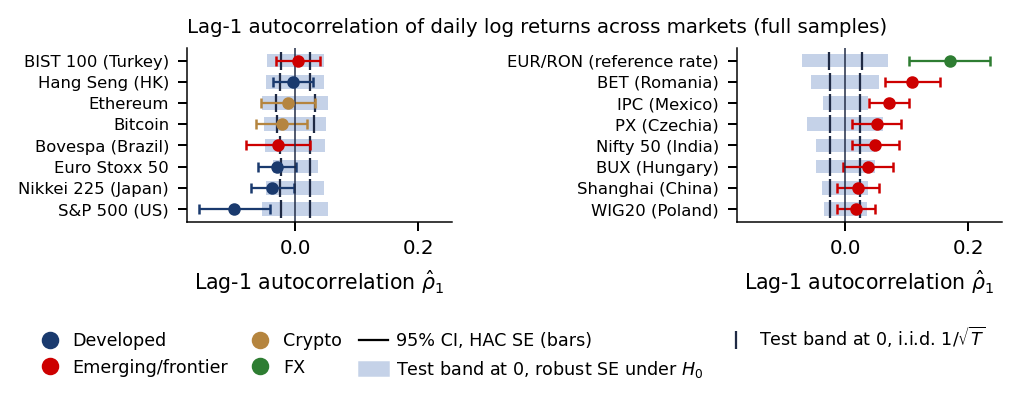
 MFM_ch2_random_walk_game
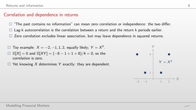
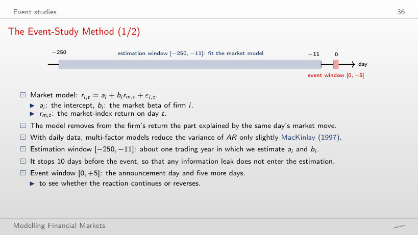
 Market Responses to ETH Development Milestones
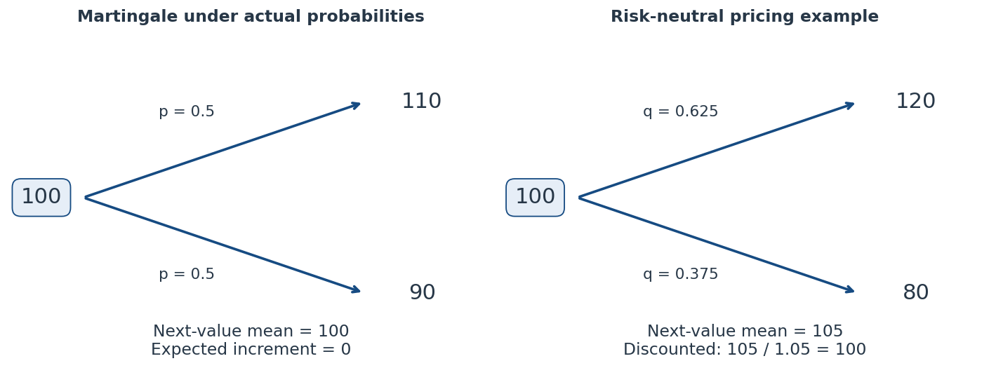 Left: the actual conditional mean stays at 100. Right: pricing probabilities give 105, whose discounted value is 100.
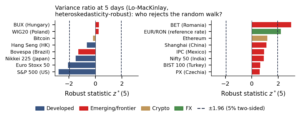
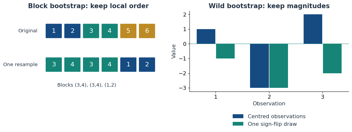 Blocks preserve local ordering; sign flips preserve absolute magnitudes. They impose different assumptions on the artificial samples.
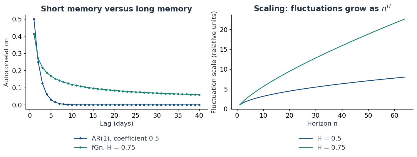 AR(1) correlations fade geometrically; the fGn example fades slowly. The right panel compares fluctuation growth across horizons.