Bucharest University of Economic Studies IDA Institute Digital Assets Blockchain Research Center AI4EFin Artificial Intelligence for Energy Finance Romanian Academy, Institute for Economic Forecasting MSCA Digital Finance
Chapter 10 measured the risk of a single position through VaR (value at risk) 1% and ES (expected shortfall) 2.5%. For a bank, this measure answers how much the bank itself can lose. Supervisors have a different concern: when does the loss of one bank become a loss of the whole financial system, with loans no longer granted and payments no longer made? This is systemic risk, and the chapter shows how it is measured from market prices.
The data of the chapter are the daily prices of 13 listed banks, six American, five European and two Romanian, from 2005 to September 2026. Four crises are visible in them: the failure of Lehman Brothers in 2008, the euro-area crisis of 2011–2012, March 2020 and March 2023. The portfolio of US banks lost 82% of its value by March 2009, and the average correlation among them rose from 0.59 in calm years to 0.94 in March 2020: in crises, several banks behave almost like a single one.
The chapter then builds the measures used by researchers and central banks: tail dependence, CoVaR and ΔCoVaR (conditional value at risk and the contribution to it), MES (marginal expected shortfall) and SRISK (systemic risk, the capital shortfall in a crisis), Granger-causality networks and Diebold–Yilmaz connectedness. The main result is that ranking banks by their own VaR 1% differs from ranking them by their contribution to the risk of the system. The chapter ends with the macroprudential tools of Basel III and the institutions that apply them in the European Union (EU) and in Romania.
Value of 100 units invested in the equally weighted portfolio of US, European and Romanian banks (the latter since 2010), on a log scale; the dotted lines mark the Lehman failure, Draghi's speech, the start of the COVID-19 (coronavirus disease 2019) crisis and the failure of SVB (Silicon Valley Bank).
Learning outcomes
Explain the channels of systemic risk and recognise them in the crises of 2008, 2011–2012, 2020 and 2023.
Estimate CoVaR 1% and ΔCoVaR by linear quantile regression and interpret them alongside VaR 1%.
Compute MES 5%, LRMES and SRISK and explain the role of leverage.
Distinguish contagion from interdependence through the Forbes–Rigobon correction and interpret an estimate of tail dependence.
Interpret a Granger-causality network and a Diebold–Yilmaz connectedness table.
Name the macroprudential tools of Basel III and the institutions that apply them in the EU and in Romania.
AI for Scientific DiscoveryAn open question about Romanian banks, the possible help of AI and the checks needed.
SummaryThe main ideas, the formulas and self-check questions.
Systemic Risk: Definition and Channels
The section defines systemic risk and explains why VaR computed separately for each bank does not capture it. It then presents the three channels through which a local problem becomes a problem of the system: direct contagion, common exposures with fire sales, and deposit withdrawals. It ends with the problem of banks too big to be allowed to fail and with a table of the measures used in the rest of the chapter.
In 2009, at the request of the G-20, the IMF (International Monetary Fund), the BIS (Bank for International Settlements) and the FSB (Financial Stability Board) defined systemic risk as the risk that the financial system as a whole stops performing its functions, namely lending, payments and trading, with large costs for the real economy (IMF, BIS & FSB, 2009). The emphasis is on functions, not institutions: the failure of a small bank whose services are taken over immediately by other banks is not a systemic event.
The same report proposes three criteria for judging whether an institution is systemically important. Size shows what share of the system's services the institution provides. Substitutability shows whether other institutions can quickly take over its activity, for example the settlement of payments or lending to a particular type of client. Interconnectedness shows how many other institutions its failure would drag down, through direct exposures or through lost confidence.
The definition yields the idea that organises the chapter: systemic risk is a property of the system, not of a single balance sheet. A bank can look safe when viewed on its own and still be dangerous for the system, because its losses arrive exactly when the other banks also lose. The measures of the following sections all try to capture this link between the bank and the system.
In brief
Systemic risk: the risk that the financial system as a whole stops working (lending, payments, trading), with large costs for the real economy IMF, BIS & FSB (2009)
the definition of the IMF (International Monetary Fund), the BIS and the FSB (Financial Stability Board) for the G-20 in 2009
The VaR 1% of a bank, defined in Chapter 10, is the loss of this bank exceeded with probability 1%. The measure looks only at the distribution of the bank's returns and says nothing about what happens to the other banks on the days when this bank is in trouble. Two banks with the same VaR 1% can have entirely different effects on the system: one loses on days when the rest of the market is calm, the other loses together with everyone else.
Regulation built only on individual VaR can even amplify risk, through a fallacy of composition. If every bank sells risky assets to reduce its own VaR, the simultaneous sales push down the prices of those assets, and the mark-to-market losses raise the risk of all. What is prudent for one bank taken separately becomes destabilising when all banks do the same. Likewise, a small bank with a large VaR can matter less for the system than a large, interconnected bank with a moderate VaR.
What is needed, therefore, are conditional measures that link the tail of the bank to the tail of the system. There are two directions. CoVaR measures the tail of the system given that the bank is in distress (Adrian & Brunnermeier, 2016). MES and SRISK measure the loss of the bank given that the market crashes; the first was proposed by Acharya, Pedersen, Philippon & Richardson (2017) and the second by Brownlees & Engle (2017). The chapter estimates both on the same 13 banks, and the difference in direction will turn out to matter.
In brief
VaR 1% of a bank (Chapter 10): the loss of this bank exceeded with probability 1%
it ignores what happens to the others when this bank is in trouble
Fallacy of composition: if every bank sells risky assets to cut its own VaR, prices fall for all and the risk of all rises
a small bank with a high VaR can matter less than a large, connected bank with a moderate VaR
We need measures of the tail of the system given the institution, or of the institution given the tail of the system
Contagion means that the failure of one institution causes losses or failures at other institutions. The most direct channel runs through the exposures between banks: interbank loans, derivative contracts in which the failed bank is the counterparty, deposits held at other banks. The banking system is thus a network of balance sheets, and a loss that wipes out the capital of one bank is passed on to its creditors, then to their creditors (Allen & Gale, 2000).
The structure of the network matters. Allen & Gale (2000) and Haldane & May (2011) show that many links have a double effect. A small shock is split among many counterparties, each loses a little, and the system absorbs it. A large shock, however, spreads along the same links to almost all institutions. The property is summarised by the phrase "robust yet fragile": the same system withstands small shocks well and gives way suddenly under large ones.
This is the origin of the idea of an institution too interconnected to fail. The problem is not its size but the number of counterparties that its failure would hit at the same time. For such an institution, the authorities have a reason to intervene even if its balance sheet is not very large, and this expectation changes its behaviour before the crisis.
In brief
Contagion: the failure of one institution causes losses or failures at others
direct exposures: interbank loans, derivatives, deposits held at other banks
a network of balance sheets: a loss travels along the links Allen & Gale (2000)
The second channel needs no direct link between banks. Common exposures arise when banks hold the same assets, for example mortgages or the bonds of the same government. A single shock to those assets hits all of them on the same day. The correlation between banks then comes from their assets, not from contracts between them.
Fire sales turn the initial loss into a spiral. A bank that must sell quickly, to cover losses or withdrawals of funding, sells below fundamental value, because the natural buyers of the asset are in trouble themselves (Shleifer & Vishny, 2011). The lower price is a loss for all holders of the asset who mark their positions to market. Brunnermeier & Pedersen (2009) describe the liquidity spiral: losses lead to higher margins demanded by creditors, higher margins lead to new sales, and the sales push prices down again.
Leverage amplifies all these mechanisms. A bank whose assets are 20 times its equity has capital equal to 5% of assets. A 5% fall in the value of the assets therefore wipes out its capital. The higher the leverage, the smaller the price fall that triggers fire sales, and this link returns in the SRISK formula of section 5.
In brief
Common exposures: banks hold the same assets (mortgages, government bonds), so one shock hits all of them at once
no link between the banks is needed: the correlation comes from the assets
Fire sales: a bank that must sell quickly sells below the fundamental value Shleifer & Vishny (2011)
the lower price is a loss for every holder of the asset (marked to market)
A bank run occurs when depositors withdraw their money at the same time, for fear that others will withdraw first (Diamond & Dybvig, 1983). The mechanism comes from the structure of a bank's balance sheet: the bank holds long-term loans that are hard to sell and owes short-term deposits that can be claimed at any moment. It cannot pay all depositors at once, even if its assets are worth more than its liabilities.
The Diamond–Dybvig model has two equilibria. If every depositor believes the others will keep their money, nobody has a reason to withdraw. If every depositor believes the others will withdraw, withdrawing becomes rational for all, and the bank, solvent at the start, ends up selling assets at a loss. Deposit insurance removes the motive to withdraw: an insured depositor gets the money back in any case, so there is no reason to run to the bank.
Information contagion extends this mechanism to other banks. The problems of one bank make investors and depositors doubt the banks that resemble it, even without any direct exposure. The photograph on the slide shows depositors queuing outside a Northern Rock branch in September 2007: it was the first run on a British bank in a century.
In brief
Bank run: depositors withdraw at once because they fear that others will withdraw first Diamond & Dybvig (1983)
a bank holds long, illiquid loans and short, liquid deposits: it cannot pay everyone at once
a run can hit a solvent bank; deposit insurance removes the reason to run
Information contagion: trouble at one bank makes investors doubt similar banks
Northern Rock (United Kingdom), September 2007: the first run on a British bank in over a century
A bank is too big to fail when its failure would hurt the economy so much that the government prefers to rescue it. If investors anticipate the rescue, the bank's creditors bear less risk than they otherwise would and ask for a lower interest rate. The bank thus receives an implicit subsidy, paid by taxpayers through the guarantee that the government provides.
The subsidy has a predictable consequence, moral hazard. Gains from risky positions stay with shareholders, while part of the losses is shared with taxpayers, so the bank has a reason to take more risk. The problem reinforces itself: the larger the bank grows, the more credible the implicit guarantee and the cheaper its funding.
After 2008, the authorities responded in two ways. Global systemically important banks, G-SIBs, are identified in a list published every year and must hold additional capital, the more so the higher their importance score (BCBS, 2018). Resolution plans must show how a bank in distress can be wound down without taxpayers' money. Measures from market data, such as CoVaR and SRISK, complement these rules: they allow banks to be ranked by systemic importance without waiting for a failure.
In brief
Too big to fail: a bank whose failure would damage the economy so much that the state rescues it
the expected rescue lowers its funding cost: an implicit subsidy
moral hazard: the bank takes more risk because losses are shared with taxpayers
The table on the slide links each measure to the question it answers. Correlation and tail dependence ask whether banks and markets crash together and are estimated from ranks, that is, from pseudo-observations, and from a t copula. CoVaR and ΔCoVaR ask how much worse the system is when a bank is in distress and are estimated by quantile regression. MES asks how much the bank loses on the market's worst days and is a conditional average.
SRISK asks how much capital the bank would miss in a crisis and combines MES with leverage. Networks ask who transmits shocks to whom, through Granger-causality tests and through the decomposition of forecast error variances. Each measure looks at the same problem from a different angle, and sections 3–6 estimate them on the same data.
All these measures use only market prices, so they are available daily for any listed bank, without waiting for accounting reports. Their weakness is shared: prices can be calm while risk builds up, as happened in 2006–2007, when low volatility made all return-based measures show low risk just before the largest crisis in the sample.
In brief
Measure
Question
Tool
correlation, tail dependence
do banks and markets crash together?
pseudo-observations, t copula
CoVaR, \(\Delta\)CoVaR
how much worse is the system when the bank is in distress?
quantile regression
MES
how much does the bank lose on the market's worst days?
conditional average
SRISK
how much capital would the bank miss in a crisis?
MES, leverage
networks
who transmits shocks to whom?
Granger tests, variance decompositions
All measures use only market prices: they are available daily, for any listed bank
Their weakness: market prices can be calm while risk builds up (2006–2007)
Section summary
Systemic risk is the risk that the financial system stops performing its functions. It arises through direct contagion, through common exposures and fire sales amplified by leverage, and through deposit runs, and individual VaR does not see it. The measures of the chapter link the tail of the bank to the tail of the system, in both directions of conditioning. The next section shows what these mechanisms look like in the data of the four crises.
Four Crises in the Data
The section describes the data of the chapter and follows the portfolios of US, European and Romanian banks from 2005 to 2026. Four episodes are analysed in turn: the failure of Lehman Brothers, the euro-area crisis, the dash for cash of March 2020 and the banking crisis of March 2023, with Silicon Valley Bank and Credit Suisse. It ends with a comparison of the four episodes in the same chart.
The sample comprises three groups of banks, each with a market index that plays the role of the system or the market. The US banks are JPMorgan Chase, Bank of America, Citigroup, Goldman Sachs, Morgan Stanley and Wells Fargo, with the S&P 500 as index. The European banks are Deutsche Bank, BNP Paribas, Santander, ING and HSBC, with the Euro Stoxx 50. The Romanian banks are Banca Transilvania (TLV) and BRD, with the BET (Bucharest Exchange Trading), the benchmark index of the Bucharest Stock Exchange (BVB). The volatility index VIX (CBOE Volatility Index) serves as an indicator of market stress.
The data are the daily adjusted closing prices of the banks and the closes of the indices, from the provider EODHD (EOD Historical Data), from January 2005 to 18 September 2026. The prices of the series being compared are first aligned on the days on which all of them have quotes, and only then are the daily log returns in percent computed, \(r_t = 100(\ln P_t - \ln P_{t-1})\). The order matters: a return computed before alignment could span two days for one series and one day for the other.
The BVB banks enter the sample in 2010, because before then many days have no trades. The days of 30–31 May 2016 are removed from the TLV series, because a price adjustment was applied one day late, an issue discussed in Chapter 2. For each group, a portfolio of banks is built with equal weights, rebalanced daily.
In brief
Group
Banks
Market index
US banks
JPMorgan Chase, Bank of America, Citigroup, Goldman Sachs, Morgan Stanley, Wells Fargo
S&P 500
European banks
Deutsche Bank, BNP Paribas, Santander, ING, HSBC
Euro Stoxx 50
Romanian banks
Banca Transilvania (TLV), BRD (since 2010)
BET
Daily adjusted closes of the banks and closes of the indices from EODHD, January 2005 – 18 September 2026; the VIX as a stress indicator
Prices are joined on common days first, then daily log returns in %: \(r_t = 100(\ln P_t - \ln P_{t-1})\)
BVB banks from 2010: before, many days have no trades; TLV without 30–31 May 2016 (a price adjustment applied one day late, Chapter 2)
Bank portfolio of a group: equal weights, rebalanced daily
Question for the room ▶ moves the investment of the 100 units to the start of 2010 (extra run). What is the maximum drawdown of the US bank portfolio?
Answer
−51%, on 23 November 2011, against −82% with the 2005 investment: the March 2009 trough is no longer in the sample. The maximum drawdown depends on the start of the sample; for the European banks the deepest point after 2010 is 21 April 2020 (−61%).
The chart shows, on a log scale, the value of 100 units invested in each of the three equally weighted portfolios: the US and European banks from 2005, the Romanian banks from 2010. On a log scale, equal vertical distances correspond to equal percentage changes, so the falls of 2008 and 2020 can be compared directly. The dotted vertical lines mark the Lehman failure, Draghi's speech of July 2012, the start of the COVID-19 crisis and the failure of SVB; a horizontal line marks the starting level of 100.
The loss measure is the maximum drawdown, the largest fall from a previous peak to a later trough. The US bank portfolio has a maximum drawdown of −82%, reached on 6 March 2009, and the European one of −76%, on 9 March 2009. The Romanian bank portfolio has a maximum drawdown of −47%, reached later, on 5 June 2012, during the euro-area crisis.
At the end of the sample, all three portfolios are above their starting value, and the Romanian one is highest. The paths there were very different, however: the European portfolio spent many years below its starting level, and the US one had to recover a loss of four fifths.
In brief
Value of 100 invested in each equal-weighted portfolio (log scale); dotted lines: Lehman, Draghi's speech, COVID-19, the failure of SVB
Maximum drawdown: US banks \(-82\%\) (6 March 2009), European banks \(-76\%\) (9 March 2009), Romanian banks \(-47\%\) (5 June 2012)
In 2008–2009, US and European banks lost about four fifths of their value. The trough did not come on the day of the Lehman failure but in March 2009, almost six months later. A systemic crisis is a process that unfolds over months: losses are discovered gradually, funding is withdrawn, fire sales continue. A risk measure that looks at a single bad day captures only the start of this process.
The European banks stayed below their 2005 level for most of the period. After 2009 came the sovereign debt crisis in the euro area and a long period of low interest rates. The Romanian banks had their largest fall in the euro-area crisis of 2011–2012, not in 2008: the parent banks of many banks in Romania are in the euro area, and doubts about them spread to the local markets.
The episodes of March 2020 and March 2023 look different. The falls were steep but short, because central banks and governments reacted within days. The difference from 2008 lies both in the larger capital of the banks and in the speed of public intervention.
In brief
2008–2009: US and European banks lost about four fifths of their value; the trough came in March 2009, six months after Lehman
a systemic crisis is a process that lasts months, not a single bad day
European banks stayed below their 2005 level for most of the period: the euro-area crisis and low interest rates
Romanian banks: their worst fall came in the euro-area crisis of 2011–2012 (the parent banks of many Romanian banks are in the euro area)
March 2020 and March 2023: sharp falls, but short; central banks and governments reacted within days
On 15 September 2008, Lehman Brothers filed for bankruptcy, the largest bankruptcy in US history, with assets of over USD 600 billion. The next day, the Federal Reserve rescued AIG (American International Group), an insurer that had sold many banks protection against default on mortgage debt. On the same day, the value of a unit of a money market fund holding Lehman paper fell below one dollar, and investors began to pull their money out of such funds, an important source of short-term funding for banks.
The episode illustrates all three channels of the previous section at once. Direct exposures arose through derivative contracts with Lehman, whose outcome was uncertain. Common exposures arose through US mortgages held by banks on both sides of the Atlantic. The withdrawal of short-term funding worked like a bank run outside classic deposits.
From the end of August to the trough in November 2008, the US bank portfolio fell by 59%, the European one by 54%, and the S&P 500 by 41%. Banks lost more than the market as a whole, a sign that they were the source of the crisis, not just its victims.
In brief
15 September 2008: Lehman Brothers files for bankruptcy, the largest bankruptcy in US history (assets above 600 billion USD)
16 September: AIG, an insurer that had sold protection on mortgage debt to many banks, is rescued by the Federal Reserve
the same day, a money market fund holding Lehman debt “breaks the buck” and investors run from such funds
All three channels at once
direct exposures (derivatives with Lehman), common exposures (mortgages), a run on short-term funding
From the end of August to the trough in November: US banks \(-59\%\), European banks \(-54\%\), S&P 500 \(-41\%\)
The euro-area crisis started in 2010 in Greece and spread to Ireland, Portugal, Spain and Italy, through doubts about the sustainability of public debt. The central mechanism was the bank–sovereign loop. Banks hold many bonds of their own government, and the government implicitly guarantees the banks. A fall in bond prices weakens the banks' capital; rescuing the banks raises government debt and lowers bond prices again.
The spiral was stopped on 26 July 2012 by a statement. Mario Draghi, President of the ECB (European Central Bank), said in London that the European Central Bank was ready to do whatever it takes to preserve the euro (Draghi, 2012). The statement was not accompanied at that moment by bond purchases; what mattered was the change in investors' expectations about what the central bank would do in the event of a new fall.
In the window July 2011 – September 2012, at the weakest point, the European bank portfolio had lost 41%, the US one 37%, and the Romanian one 34%. The fact that US banks also fell sharply shows how closely the global banking system was tied to the fate of the euro area.
In brief
Greece (2010), then Ireland, Portugal, Spain and Italy: doubts about government debt
the bank–sovereign loop: banks hold their own government's bonds, and the government stands behind its banks
a fall in bond prices weakens the banks; rescuing the banks weakens the state
26 July 2012: Mario Draghi, President of the ECB (European Central Bank): “the ECB is ready to do whatever it takes to preserve the euro” Draghi (2012)
a promise, not a purchase, stopped the spiral: the role of expectations
July 2011 – September 2012, worst point: European banks \(-41\%\), US banks \(-37\%\), Romanian banks \(-34\%\)
In March 2020, the restrictions imposed by the COVID-19 pandemic made firms, funds and investors want liquidity at the same time. The episode is known as the dash for cash: not only shares but even government bonds, usually the investors' refuge, were sold. The stress started outside the banks, in funds, in firms that had lost their revenues, and in the bond market.
Banks were better capitalised than in 2008, thanks to the Basel III rules, and became part of the solution: firms drew on the credit lines they already had at banks, and banks were able to honour them. The authorities reacted quickly. Central banks bought assets, and the Federal Reserve lent dollars to other central banks, so that banks outside the United States could fund their dollar positions.
At the trough of 23 March 2020, the US bank portfolio had lost 48%, the European one also 48%, the Romanian one 35%, and the S&P 500 34%. The image of New York's financial district, empty on 25 March 2020, sums up the nature of the episode: a shock coming from the real economy, not from bank balance sheets.
In brief
COVID-19 lockdowns: everyone wanted cash at the same time, even government bonds were sold
the stress started outside the banks: funds, firms, the bond market
banks were better capitalised than in 2008 (Basel III) and became part of the solution (credit lines)
Fast policy response: central banks bought assets and lent in dollars to other central banks
trough on 23 March 2020: US banks \(-48\%\), European banks \(-48\%\), Romanian banks \(-35\%\), S&P 500 \(-34\%\)
SVB had an unusual business model. Its deposits came mostly from technology firms, and most of them exceeded the insured limit. The bank invested them largely in long-term bonds. The rise in interest rates in 2022 lowered the price of these bonds and produced large unrealised losses, which would become real if the bank had to sell.
On 9 March 2023, depositors tried to withdraw about USD 42 billion in a single day, and on 10 March the bank was closed (Federal Reserve, 2023; FDIC, 2023). It was a bank run in the age of banking apps, faster than any before: uninsured depositors, well informed and connected to each other, could act within hours.
SVB was a mid-sized bank, not among the institutions regarded as systemic. It became systemic through information contagion: investors looked for banks with the same weaknesses, uninsured deposits and unrealised losses on bonds, and other US regional banks fell sharply in the following days.
In brief
SVB (Silicon Valley Bank): deposits of technology firms, mostly above the insured limit, invested in long-term bonds
rising interest rates in 2022 created large unrealised losses on the bonds
9 March 2023: depositors tried to withdraw about 42 billion USD in one day; 10 March: the bank is closed Federal Reserve (2023); FDIC (2023)
A run in the age of mobile banking: faster than any run before
a mid-sized bank became systemic through information contagion: other regional banks fell the next days
Credit Suisse was a G-SIB that had been losing clients and money for years, after scandals and large losses with hedge-fund clients. After the failure of SVB, its investors and depositors left quickly, and the bank came to the brink of failure within days. The episode shows that a weakened bank is the most exposed to information contagion from another bank, even without direct links between them.
On 19 March 2023, Credit Suisse was taken over by UBS, with the approval of the Swiss supervisory authority FINMA (Eidgenössische Finanzmarktaufsicht) (FINMA, 2023). AT1 (additional tier 1) bonds of about CHF 16 billion were written off. These instruments are designed precisely to absorb losses, and writing them off showed that they can do so in practice.
The solution was nevertheless a rescue by merger, not a resolution of the kind promised after 2008: the too-big-to-fail problem had not gone away. From the end of February to the trough, the European bank portfolio lost 21%, the US one 16%, and the Romanian one 7%.
In brief
Credit Suisse: a G-SIB that had lost clients and money for years (scandals, losses on hedge-fund clients)
after SVB, investors and depositors left quickly
19 March 2023: takeover by UBS, approved by the Swiss supervisor FINMA FINMA (2023)
AT1 bonds (additional tier 1 capital) of about 16 billion CHF were written down to zero
a rescue by merger, not a resolution: too big to fail was still alive
From the end of February to the trough: European banks \(-21\%\), US banks \(-16\%\), Romanian banks \(-7\%\)
Question for the room ▶ moves the start of each window 30 days later (extra run). What becomes of the minimum of the US banks in the March 2020 episode?
Answer
−10.8% instead of −47.6%: the window starts on 15 March 2020, after most of the fall, and the portfolio ends at +16.9%. The cumulative return is measured from the start of the window, so the comparison of episodes depends on that date.
The chart has four panels, one for each crisis: Lehman in 2008 (September–December), the euro area (July 2011 – September 2012), March 2020 and March 2023. In each panel, the vertical axis shows the cumulative return in percent from the start of the window, for the US bank portfolio, the European bank portfolio, the S&P 500 and, from the euro-area crisis onwards, the Romanian bank portfolio.
The comparison separates banking crises from the others. In 2008 and in 2011–2012, banks fell much more than the S&P 500: banks were the problem. In March 2020, banks fell together with the market, because the shock came from outside the banking system. In March 2023, banks fell while the S&P 500 rose: a crisis confined to the banking sector, which did not contaminate the rest of the market.
The difference has consequences for measurement. A measure that compares the bank with the market will see in 2008 and in 2023 banks that move worse than the market, and in 2020 banks that move together with the market. The following sections turn these observations into measures.
In brief
Cumulative return from the start of each window; the Romanian banks enter the data in 2010
Interpretation: in 2008 and 2011–2012 the banks fell much more than the S&P 500 (the banks were the problem); in 2020 they fell with the market; in 2023 they fell while the market rose
The four crises show all channels of systemic risk: direct and common exposures in 2008, the bank–sovereign loop in the euro area, a liquidity shock from outside the banks in 2020, and information contagion in 2023. US and European banks lost about four fifths of their value in 2008–2009, with the trough six months after Lehman, while the rapid interventions of 2020 and 2023 shortened the falls. The next section measures how much banks move together in these periods.
Correlation and Tail Dependence in Crises
The section measures how much banks move together and how this comovement changes in crises. It starts from rolling correlations, shows why a higher correlation does not prove contagion (the Forbes–Rigobon correction), and then turns to tail dependence, which looks only at bad days, estimated empirically and from a t copula.
Mean of the average pairwise correlation by period (the numbers of the previous slide)
Question for the room ▶ goes through the years 2005–2026. In which year is the yearly mean of the TLV–BRD correlation highest?
Answer
In 2019: 0.80, above 2020 (0.76) and 2011 (0.56). The 120-day correlation of two stocks is noisy and can peak in a calm year, as the daily maximum of 9 May 2019 also shows.
Question for the room ▶ picks the March 2020 crisis (extra run). Does the corrected correlation ρ* exceed the calm-period correlation of 0.40?
Answer
No: ρ_crisis = 0.74, but the variance of the US portfolio rises 47-fold (δ = 46.0), so ρ* = 0.74/√(1 + 46.0 × 0.451) = 0.16. Of the four windows only March 2023 gives ρ* = 0.42, just above 0.40, because volatility rose little (δ = 3.7).
Question for the room With a 60-day window (▶, extra run), where does the maximum correlation of TLV and BRD go?
Answer
To 0.96, on 6 February 2019, still outside any crisis (with 120 days: 0.93 on 9 May 2019). For a single pair of stocks a short window gives larger extremes; the maximum of the US banks stays on 16 March 2020 (0.95).
The chart shows, for each group of banks, the average of the pairwise correlations between banks, computed on daily returns in rolling windows of 120 days. The vertical axis runs from 0 to 1, and the dotted lines mark the same four events as in the previous section. For the Romanian banks, the average is simply the correlation between TLV and BRD.
For the US banks, the average correlation was 0.59 before the crisis, between July 2005 and June 2007, and reached its maximum of 0.94 on 16 March 2020. For the Romanian banks, the variation is even larger: the correlation between TLV and BRD was 0.31 in 2017 and rose to 0.85 in April–June 2020. The Romanian series is also the most unstable of the three, with wide rises and falls from one year to the next: its maximum, 0.93 on 9 May 2019, falls outside any crisis.
The rolling correlation shows that the link between banks is not constant. In calm years, each bank responds partly to its own news; in a crisis, the same common factor dominates the returns of all.
In brief
Average of the pairwise correlations of daily returns within each group, on 120-day windows
US banks: \(0.59\) before the crisis (July 2005 – June 2007), up to \(0.94\) (16 March 2020); TLV and BRD: \(0.31\) in 2017, \(0.85\) in April–June 2020, maximum \(0.93\) (9 May 2019)
When the average correlation approaches 1, a portfolio of several banks behaves almost like a single bank. The benefit of diversification, which rests on the losses of one bank being offset by the gains of another, disappears exactly in the period when it would be most useful. The cause is the common factor: the market as a whole and funding stress dominate the news specific to each bank.
The case of the two Romanian banks is the clearest, with one caveat: the series reaches its maximum, 0.93, on 9 May 2019, outside any crisis, so for two stocks a single peak says little. In calm years, BVB shares are driven by each company's own news and by low liquidity: days without significant trades or with small volumes add independent noise to each series and lower the correlation. In a crisis, the common shock is large enough to drown this noise, and the correlation jumps.
Two precautions are needed. A correlation estimated over 120 days has a large estimation error, so small movements of the line should not be interpreted; with only two stocks, as for TLV and BRD, even a peak can come in a calm year. And a rise in correlation does not, on its own, prove that the link between banks has strengthened: it can also appear only because volatility has risen, as the next slide shows.
In brief
In crises, the banks move together: a portfolio of several banks is almost one bank
the common factor (the market, funding stress) dominates the bank-specific news
The two Romanian banks: low correlation in 2017, very high in 2020; the maximum (9 May 2019) falls outside any crisis
in calm years the BVB stocks are driven by their own news and by low liquidity; in a crisis, by the common shock
Caution: a rolling correlation estimated on 120 days is noisy (for two stocks, it can peak in a calm year), and a rise in correlation does not prove contagion (next slide)
Contagion and Interdependence: Forbes and Rigobon (1/2)
Forbes & Rigobon (2002) start from a simple model, \(y = \beta x + e\), in which \(x\) is the return of the source market, \(y\) the return of the other market, \(\beta\) the strength of the link, and \(e\) a shock to \(y\) unrelated to \(x\). The correlation between \(x\) and \(y\) is \(\rho = \beta\sigma_x/\sqrt{\beta^2\sigma_x^2 + \sigma_e^2}\). If the variance of \(x\) rises while \(\beta\) and \(\sigma_e\) stay the same, the correlation rises automatically, because the common part of \(y\) becomes larger relative to its own noise.
A higher correlation in a crisis can therefore be the same link, seen in a more volatile period. Forbes and Rigobon call this case interdependence. Contagion, in their sense, means that the link itself, \(\beta\), becomes stronger in the crisis. To separate the two cases, the crisis correlation is recomputed at the volatility of the calm period:
In (15.1),\(\rho\) is the correlation measured in the crisis, \(\sigma^2\) is the variance of the source market in each period, and \(\delta\) is the relative increase in this variance. The corrected correlation \(\rho^*\) is compared with the correlation of the calm period, \(\rho_{\text{calm}}\): if \(\rho^* > \rho_{\text{calm}}\), the link has strengthened and the data point to contagion; otherwise, the rise in correlation is explained by volatility.
In brief
If \(y = \beta x + e\) with fixed \(\beta\), the correlation of \(x\) and \(y\) rises automatically when the variance of \(x\) rises Forbes & Rigobon (2002)
\(x\): the return of the source market; \(y\): the return of the other market; \(\beta\): the strength of the link; \(e\): a shock of \(y\) unrelated to \(x\)
a higher correlation in a crisis may be the same link seen in a more volatile period: interdependence
The example applies the correction to the US bank portfolio, as the source, and the European bank portfolio. The calm period is January 2005 – June 2007, with 506 days, and the crisis is 15 September – 31 December 2008, with 72 days. The correlation rises from 0.40 in the calm period to 0.60 in the crisis, a rise that, taken alone, would suggest contagion.
The daily variance of the US portfolio, however, rose from 0.89 to 75.4, so \(\delta = 83.7\). With \(1 - \rho^2 = 0.638\), the corrected correlation is \(\rho^* = 0.60/\sqrt{1 + 83.7 \times 0.638} = 0.60/\sqrt{54.4} = 0.08\). After the correction, the crisis correlation is no longer larger than the calm one, but much smaller.
The interpretation is that the data are consistent with interdependence, not with a stronger link between US and European banks. The conclusion must be read with care: the correction assumes the linear model above and an own shock \(e\) with the same variance in both periods. It shows, however, how much a naive comparison of correlations can exaggerate when volatility rises almost 85-fold.
In brief
Worked example
US bank portfolio (source) and European bank portfolio: calm January 2005 – June 2007 (\(n = 506\)), crisis 15 September – 31 December 2008 (\(n = 72\))
Correlation describes the whole joint distribution, including ordinary days. For systemic risk, however, what matters are the bad days, and these are better studied through pseudo-observations. For each series, the return of a day is replaced by its rank among the \(n\) returns of the series, divided by \(n + 1\):\(U = \text{rank}/(n + 1)\). The values of \(U\) lie in \((0, 1)\), and \(U \le 0.05\) means that the day is one of the worst 5% of the days of the series. The marginal distributions no longer matter: only the dependence structure remains, that is, the copula of Chapter 10.
Lower tail dependence at level \(q\) is the conditional probability
\[\lambda(q) = P(U_1 \le q \mid U_2 \le q),\]
(15.2)
where \(U_1\) is the pseudo-observation of the bank and \(U_2\) that of the market. \(\lambda(q)\) is the probability that the bank is in its worst \(q\) of days, given that the market is in its worst \(q\) of days. If the bank and the market were independent, \(\lambda(q) = q\); if they moved perfectly together, \(\lambda(q) = 1\).
The limit \(\lambda_L = \lim_{q \to 0}\lambda(q)\) is the tail dependence coefficient. It tells whether extreme crashes of the two series tend to occur together even at the farthest levels of the tail. For systemic risk, this measure is more relevant than correlation: it tells how often a bank and the market are together in their worst days.
In brief
Pseudo-observations: \(U = \text{rank}/(n + 1)\), the rank of a return among the \(n\) returns of its series, scaled to \((0, 1)\)
\(U \le 0.05\): one of the worst 5% of days of that series; the marginal distributions no longer matter
\(U_1\): the bank; \(U_2\): the market; \(\lambda(q)\): the probability that the bank is in its worst \(q\) days, given that the market is in its worst \(q\) days
under independence \(\lambda(q) = q\); the limit \(\lambda_L = \lim_{q \to 0}\lambda(q)\) is the tail-dependence coefficient
For systemic risk: tail dependence measures how often a bank and the market are in their worst days together
The limit \(\lambda_L\) cannot be estimated directly from the data, because at very small \(q\) too few days remain. It is obtained from a parametric copula. The Gaussian copula has \(\lambda_L = 0\) for any correlation below 1: extreme crashes become, in the limit, independent. The t copula, by contrast, has a positive tail dependence coefficient (Demarta & McNeil, 2005):
In (15.3),\(t_{\nu+1}\) is the distribution function of the Student-t distribution with \(\nu + 1\) degrees of freedom, \(\rho\) is the correlation parameter of the copula, and \(\nu\) its degrees of freedom. The coefficient rises when \(\rho\) rises and when \(\nu\) falls: a small \(\nu\) means strong joint crashes, and as \(\nu \to \infty\) the t copula becomes Gaussian and \(\lambda_L \to 0\).
Estimation has two steps. The parameter \(\rho\) is obtained from Kendall's \(\tau\), a rank correlation, through \(\rho = \sin(\pi\tau/2)\);\(\tau = (C - D)/\binom{n}{2}\), where \(C\) and \(D\) are the numbers of concordant and discordant pairs of days, that is, pairs in which the two series move in the same direction or in opposite directions. The degrees of freedom \(\nu\) are then estimated by maximum likelihood, with \(\rho\) held fixed.
In brief
The t copula (Chapter 10) has a positive tail-dependence coefficient Demarta & McNeil (2005); the Gaussian copula has \(\lambda_L = 0\)
\(t_{\nu+1}\): the distribution function of a Student-t with \(\nu + 1\) degrees of freedom
\(\rho\): the correlation parameter of the copula; \(\nu\): its degrees of freedom; a small \(\nu\) gives strong joint crashes
Estimation
\(\rho = \sin(\pi\tau/2)\) from Kendall's \(\tau\), a rank correlation; \(\nu\) by maximum likelihood
\(\tau = (C - D)/\binom{n}{2}\); \(C\), \(D\): the numbers of concordant and discordant pairs of days (both series move in the same or in opposite directions)
The table applies these estimates to four pairs. For the US bank portfolio and the S&P 500, with 5,229 days, the correlation is 0.79, \(\lambda(5\%) = 0.64\) and \(\lambda(1\%) = 0.63\), and the t copula gives \(\hat\nu = 3.2\) and \(\lambda_L = 0.49\). For the European banks and the Euro Stoxx 50, the values are even higher: correlation 0.86, \(\lambda(5\%) = 0.72\),\(\lambda(1\%) = 0.67\),\(\hat\nu = 3.1\) and \(\lambda_L = 0.59\). For the Romanian banks and the BET, with 3,414 days, the correlation is 0.86, \(\lambda(5\%) = 0.65\),\(\lambda(1\%) = 0.62\),\(\hat\nu = 4.3\) and \(\lambda_L = 0.53\).
The values must be compared with those under independence, \(\lambda(5\%) = 0.05\) and \(\lambda(1\%) = 0.01\). On more than half of the market's worst days, the banks are also in their worst days. The small degrees of freedom, between 3 and 4, mean strong joint crashes, which a Gaussian copula would miss entirely. The fourth pair, European and US banks, has lower dependence: correlation 0.59, \(\lambda(5\%) = 0.43\),\(\lambda(1\%) = 0.50\) and \(\lambda_L = 0.36\), partly because trading hours differ.
The empirical estimate \(\lambda(1\%)\) rests on a few dozen days, so it is imprecise: for the European–US pair, it even comes out larger than \(\lambda(5\%)\). The t-copula estimate uses all the data, at the price of an assumption about the form of the dependence.
In brief
Pair
\(n\)
corr.
\(\lambda(5\%)\)
\(\lambda(1\%)\)
\(\hat\nu\)
\(\lambda_L\) (t)
US banks, S&P 500
5 229
\(0.79\)
\(0.64\)
\(0.63\)
\(3.2\)
\(0.49\)
European banks, Euro Stoxx 50
5 212
\(0.86\)
\(0.72\)
\(0.67\)
\(3.1\)
\(0.59\)
Romanian banks, BET
3 414
\(0.86\)
\(0.65\)
\(0.62\)
\(4.3\)
\(0.53\)
European banks, US banks
4 895
\(0.59\)
\(0.43\)
\(0.50\)
\(3.0\)
\(0.36\)
\(\lambda(q)\): empirical; \(\hat\nu\) and \(\lambda_L\): t copula; under independence \(\lambda(5\%) = 0.05\) and \(\lambda(1\%) = 0.01\)
Interpretation: on more than half of the market's worst days the banks are also in their worst days; the small \(\hat\nu\) (about 3–4) means strong joint crashes, which a Gaussian copula misses entirely
\(\lambda(1\%)\) rests on a few dozen days: an imprecise estimate
Tail dependence (the table of the slide and λ(q) at the chosen level)
Question for the room ▶ lowers q to 0.5% (extra run). What happens to λ(q) for the US banks and the S&P 500?
Answer
It rises to 0.73, from 0.64 at 5%; under independence it would be 0.005. The estimate rests on the 26 worst days of the S&P 500, so it is imprecise: for the European banks λ(0.5%) falls to 0.58.
Question for the room At q = 1% (▶, extra run), how many times as many joint bad days do the US banks and the S&P 500 have as under independence?
Answer
About 63 times: 33 days against q²n = 0.0001 × 5,229 = 0.52, against 12.7 times at q = 5%. The ratio grows towards the tail: very bad days come together.
The chart shows, in two panels, the lower-left corner of the cloud of pseudo-observations: on the horizontal axis, the pseudo-observation of the index (S&P 500 and BET, respectively), on the vertical axis, that of the bank portfolio, both between 0 and 0.3. The orange points are the days on which both the bank portfolio and the index are in their worst 5% of days, that is, the points in the square \([0, 0.05] \times [0, 0.05]\).
For the US banks there are 166 such joint days, against 13 under independence, about 13 times as many. For the Romanian banks, the number is 110, against 9 under independence. The number expected under independence is \(n \times 0.05 \times 0.05\): any day has probability 0.05 of being bad for each series, and under independence the probabilities multiply.
The picture makes the measure \(\lambda(5\%)\) of the previous table concrete. The orange square is almost full, and the cloud of points narrows towards the lower-left corner: when the market has a very bad day, banks very rarely have a good one.
In brief
Lower-left corner of the pseudo-observations; orange: both the bank portfolio and the index in their worst 5% of days
US: 166 joint bad days against 13 under independence (about 13 times more); Romania: 110 against 9
In crises, correlations between banks rise, and diversification across banks loses its effect. The Forbes–Rigobon correction shows, however, that much of the rise can come from volatility: for US and European banks in 2008, the corrected correlation falls from 0.60 to 0.08. Tail dependence confirms that banks and markets fall together: on more than half of the market's worst days, the banks are also in their worst days. The next section turns this link between tails into a measure of each bank's contribution.
CoVaR and Delta-CoVaR
The section defines CoVaR, the VaR of the system conditional on the state of an institution, and ΔCoVaR, the institution's contribution to systemic risk. It estimates them by quantile regression for JPMorgan Chase and for all 13 banks, compares ΔCoVaR with the bank's own VaR and builds a time-varying version. It ends with the paper of Adrian and Brunnermeier.
Let \(X^i\) be the return of institution \(i\) and \(X^{sys}\) the return of the system. For the level \(\alpha\), the tail probability, \(q_\alpha(X^i)\) is the \(\alpha\)-quantile of \(X^i\), and \(\mathrm{VaR}^i_\alpha = -q_\alpha(X^i)\) is the loss of \(i\) exceeded with probability \(\alpha\), as in Chapter 10. Adrian & Brunnermeier (2016) define CoVaR as the VaR of the system on a day when the institution is exactly at its own VaR:
In (15.4),\(q_\alpha(X^{sys} \mid \cdot)\) is the \(\alpha\)-quantile of the system's return, conditional on the event after the bar. For \(\alpha = 1\%\), the measure is the VaR 1% of the system on a day when institution \(i\) is at its own VaR 1%, and it is called "CoVaR 1%".
CoVaR alone mixes two things: the risk of the system in general and the effect of the institution. The institution's contribution is isolated by the difference between the distress state and an ordinary day for the institution:
where \(q_{50\%}\) is the median of \(X^i\). ΔCoVaR tells how much the VaR of the system rises when the institution moves from an ordinary day to a distress day. The reference is the median, not the mean, because the median describes a typical day and is not affected by the tails.
In brief
\(X^i\): return of institution \(i\); \(X^{sys}\): return of the system; level \(\alpha\) = probability of the tail (Chapter 10)
\(q_\alpha(X^i)\): the \(\alpha\)-quantile of \(X^i\); \(\mathrm{VaR}^i_\alpha = -q_\alpha(X^i)\): the loss of \(i\) exceeded with probability \(\alpha\)
The estimation tool is the linear quantile regression of Koenker & Bassett (1978), met in Chapter 13 for VaR 1%. It models the conditional quantile directly, \(q_\alpha(Y \mid X = x) = a_\alpha + b_\alpha x\), with intercept \(a_\alpha\) and slope \(b_\alpha\). The coefficients are estimated by minimising the quantile loss:
Here \(u\) is the residual, and \(\mathbf{1}\{u < 0\}\) is 1 if the point lies below the line and 0 otherwise. A positive residual costs \(\alpha u\), a negative one costs \((1 - \alpha)|u|\). For \(\alpha = 1\%\), a point below the line costs 99 times as much as one at the same distance above it, so the minimum is reached when the line passes below about 99% of the points.
The idea is the same as in Chapter 13, where the explanatory variable was a measure of past volatility. Here the explanatory variable is the return of another institution on the same day. The slope \(b_\alpha\) can differ from the OLS (ordinary least squares) slope: the tail of the system's distribution can react to the institution more strongly or more weakly than its centre, and quantile regression captures exactly this difference.
In brief
Linear quantile regression Koenker & Bassett (1978): \(q_\alpha(Y \mid X = x) = a_\alpha + b_\alpha x\)
\(a_\alpha\): the intercept (constant term); \(b_\alpha\): the slope
estimated by minimising \(\sum_t \rho_\alpha(y_t - a - bx_t)\), with the check loss \(\rho_\alpha(u) = u(\alpha - \mathbf{1}\{u < 0\})\)
\(u\): the residual; \(\mathbf{1}\{u < 0\}\): 1 if the point is below the line, 0 otherwise
for \(\alpha = 1\%\), a residual below the line costs 99 times more than one above it: the line passes below 99% of the points
Same idea as VaR 1% by quantile regression in Chapter 13, now with another institution as the regressor
the slope \(b_\alpha\) can differ from the OLS slope: the tail can react more strongly than the centre
The first step is the quantile regression of the system's return on the institution's return at level \(\alpha\):\(X^{sys}_t = a + bX^i_t + \varepsilon_t\)(Adrian & Brunnermeier, 2016). It yields the estimated intercept \(\hat a\) and the estimated slope \(\hat b\). By construction, the \(\alpha\)-quantile of the error \(\varepsilon_t\) is zero, so \(\hat a + \hat b x\) is the \(\alpha\)-quantile of the system on a day when the institution has return \(x\).
The second step estimates two empirical quantiles of the institution: \(\hat q_\alpha(X^i)\), the distress state, and \(\hat q_{50\%}(X^i)\), the median. The third step plugs them into the regression line:
In the ΔCoVaR formula, the intercept drops out: only the slope and the distance between the institution's two quantiles matter. An institution has a large ΔCoVaR either because the system reacts strongly to it (large slope) or because its returns have a long tail (large distance between the median and the 1% quantile). In this chapter, the system is approximated by the region's stock index, the S&P 500, the Euro Stoxx 50 or the BET; Adrian and Brunnermeier use the portfolio of all financial institutions.
In brief
Step 1: quantile regression of the system on the institution at level \(\alpha\): \(X^{sys}_t = a + bX^i_t + \varepsilon_t\)Adrian & Brunnermeier (2016)
\(\hat a\), \(\hat b\): the estimated intercept and slope; the \(\alpha\)-quantile of the error \(\varepsilon_t\) is zero by construction
Step 2: the empirical quantiles of the institution: \(\hat q_\alpha(X^i)\) (distress) and \(\hat q_{50\%}(X^i)\) (median)
Step 3: plug in
\(\mathrm{CoVaR}_\alpha = -(\hat a + \hat b\,\hat q_\alpha(X^i))\)
\(\Delta\mathrm{CoVaR}_\alpha = \hat b\,\big(\hat q_{50\%}(X^i) - \hat q_\alpha(X^i)\big)\): only the slope and the distance between the two quantiles matter
Here the system is proxied by the regional equity index (S&P 500, Euro Stoxx 50, BET); Adrian and Brunnermeier use the portfolio of all financial institutions
The example uses the daily log returns of JPMorgan Chase (JPM) and the S&P 500 from 2005 to 2026, \(n = 5{,}229\) days. The quantile regression at 1% gives \(\hat a = -2.35\) and \(\hat b = 0.39\). The 1% quantile of JPM is \(\hat q_{1\%} = -6.27\%\), so the VaR 1% of JPM is 6.27%, and the median of JPM is \(\hat q_{50\%} = 0.07\%\).
CoVaR 1% is \(-(-2.35 + 0.39 \times (-6.27)) = 2.35 + 2.445 = 4.795\%\), computed from the estimates rounded as displayed; the unrounded estimates give 4.79%, the value in the chart. On an ordinary day for JPM, at its median, the same line gives a CoVaR of 2.32%. The difference is ΔCoVaR 1% \(= 0.39 \times (0.07 - (-6.27)) = 0.39 \times 6.34 = 2.47\%\). For comparison, the unconditional VaR 1% of the S&P 500 is 3.53%.
The interpretation: when JPM is in distress, the daily loss of the index exceeded with probability 1% is 4.79%, against 2.32% on an ordinary day for JPM. The state of the bank shifts the tail of the system by almost 2.5 percentage points. The unconditional VaR of the S&P 500, 3.53%, lies between the two values, because it does not condition on the state of JPM.
In brief
Daily log returns, 2005–2026 (\(n = 5\,229\)); quantile regression at 1%: \(\hat a = -2.35\), \(\hat b = 0.39\)
JPM: \(\hat q_{1\%} = -6.27\%\) (so VaR 1% of JPM \(= 6.27\%\)), median \(\hat q_{50\%} = 0.07\%\)
Question for the room ▶ moves to α = 5% (extra run). Is the CoVaR 5% of the S&P 500 conditional on JPM larger or smaller than 4.79%?
Answer
Smaller: 2.45%. The JPM quantile (−3.07%) and the intercept (−1.26) are less extreme, and the slope stays 0.39; ΔCoVaR 5% = 1.22%, about half of 2.47%.
Question for the room ▶ goes through α = 2.5%, 5% and 10% (extra run). How does the slope b̂ of the red line change for JPM?
Answer
Hardly at all: 0.385, 0.390 and 0.401, against 0.390 at 1% and 0.398 at the median. The intercept moves, from −2.35 to −0.86: the lines are almost parallel, so ΔCoVaR falls because the distance between the JPM quantiles falls.
The chart is a scatter of daily returns: on the horizontal axis the log return of JPM, on the vertical axis that of the S&P 500, both in percent. The red line is the 1% quantile regression line, \(-2.35 + 0.39x\), and the green line is the median regression line, \(0.04 + 0.40x\). Two dashed vertical lines mark the 1% quantile of JPM, at −6.27%, and the median of JPM, at 0.07%.
The red dot lies on the red line, above the 1% quantile of JPM: its ordinate is minus CoVaR 1%, about −4.8%. The green square also lies on the red line, but above the median of JPM: its ordinate, −2.32%, is minus CoVaR at the median. ΔCoVaR is the vertical distance between the red dot and the green square, 2.47%.
The picture shows why only the slope matters: both points lie on the same line, and the vertical distance between them is the slope times the horizontal distance. The two lines have almost equal slopes, 0.39 and 0.40, so for JPM the tail of the index reacts to the bank about as much as its centre does; the difference between them is only a vertical shift.
In brief
Red line: the 1% quantile of the S&P 500 given JPM; green line: the median; dashed: the 1% quantile and the median of JPM
\(\Delta\)CoVaR is the vertical distance between the red dot and the green square on the red line: \(2.47\%\)
Question for the room At α = 5% (▶, extra run), what is the ΔCoVaR of TLV?
Answer
1.51%, less than half of 3.31%: the slope falls from 0.611 to 0.542 and the distance between TLV’s median and its quantile falls from 5.41 to 2.79 percentage points; 0.542 × 2.79 = 1.51.
Question for the room At the 5% level (▶, extra run), which group of banks has the largest ΔCoVaR?
Answer
Still the European banks: 1.43–1.68% (Santander 1.68%), against 1.12–1.33% for the US banks; TLV 1.51%, BRD 1.45%. At 1% the largest value was TLV’s (3.31%).
The chart shows as bars the ΔCoVaR 1% of each of the 13 banks, with the system given by the region's index: blue for the US banks (S&P 500), red for the European ones (Euro Stoxx 50) and green for the Romanian ones (BET). Each bar has a 95% confidence interval obtained by a moving block bootstrap: blocks of 20 consecutive days are resampled, 200 times, to preserve the time dependence of returns.
The US banks have values between 2.1% and 2.5%, the European banks between 2.9% and 3.2%, and the Romanian banks have TLV at 3.31% and BRD at 3.05%. The largest value of all is that of Banca Transilvania. The intervals are wide: for TLV, the widest of all, they run from about 2.3% to almost 4.8%.
In brief
System: the regional index; 95% intervals from a moving-block bootstrap (blocks of 20 days, 200 resamples)
US banks: 2.1–2.5%; European banks: 2.9–3.2%; TLV \(3.31\%\), BRD \(3.05\%\); largest: Banca Transilvania
The confidence intervals overlap heavily within each region, so the data cannot rank the banks precisely by systemic importance. A ranking published without its uncertainty would give false precision: the difference between first and fourth place can be smaller than the estimation error. Like any estimate, a ranking must come with its interval, obtained here by the bootstrap, a method introduced in Chapter 2.
The European and Romanian banks have a larger ΔCoVaR than the US banks. Part of the difference comes from how the system is built. Banks have a larger weight in the Euro Stoxx 50 and in the BET than in the S&P 500, so the European and Romanian indices are closer to a banking system. Moreover, TLV and BRD are among the largest stocks in the BET, so the BET partly measures them.
The ranking of the banks is, however, robust to the chosen level. ΔCoVaR computed at 5% ranks the banks almost as at 1%: the Spearman correlation between the two rankings is 0.87. Spearman's rank correlation is \(\rho_S = 1 - 6\sum_i d_i^2/(N(N^2 - 1))\), where \(d_i\) is the difference between the two ranks of bank \(i\) and \(N\) the number of banks; it is 1 for identical rankings and −1 for reversed rankings.
In brief
The intervals overlap: within a region, the data cannot rank the banks precisely
a ranking of systemic importance needs its uncertainty, like any estimate (bootstrap, Chapter 2)
European and Romanian banks have a larger \(\Delta\)CoVaR than US banks
banks weigh more in the Euro Stoxx 50 and in the BET than in the S&P 500: the index is closer to a banking system
TLV and BRD are among the largest stocks of the BET, so the BET partly measures themselves
Robustness: the ranking at 5% is close to the ranking at 1% (Spearman correlation \(0.87\))
Spearman: the correlation of the ranks, \(\rho_S = 1 - 6\sum_i d_i^2/(N(N^2 - 1))\); \(d_i\): the difference of the two ranks of bank \(i\); \(N\): the number of banks
The second example uses TLV and the BET, with daily log returns since 2010, \(n = 3{,}414\) days. The quantile regression at 1% gives the slope \(\hat b = 0.61\), much larger than that of JPM on the S&P 500. The 1% quantile of TLV is \(\hat q_{1\%} = -5.23\%\), so the VaR 1% of TLV is 5.23%, and the median of TLV is 0.18%.
ΔCoVaR 1% is \(0.61 \times (0.18 + 5.23) = 3.31\%\), and the CoVaR 1% of the BET is 5.28%. The 95% block-bootstrap confidence interval for ΔCoVaR is [2.35, 4.78]. Although the VaR 1% of TLV is smaller than that of JPM, the ΔCoVaR of TLV is larger, because of the slope.
The interpretation: a distress day for TLV lowers the 1% quantile of the BET by about 3.31 percentage points. Part of this effect is mechanical, however: TLV has one of the largest weights in the BET, so a fall in TLV is, by construction, a fall in the index. A cleaner system would be the BET without TLV, and the difference between the two estimates would show how much of ΔCoVaR is an economic link and how much is the composition of the index.
In brief
TLV and the BET, daily log returns since 2010 (\(n = 3\,414\)); quantile regression at 1%: \(\hat b = 0.61\)
TLV: \(\hat q_{1\%} = -5.23\%\) (VaR 1% of TLV), median \(0.18\%\)
\(\Delta\)CoVaR 1% \(= 0.61 \times (0.18 + 5.23) = 3.31\%\); CoVaR 1% of the BET \(= 5.28\%\)
95% block-bootstrap interval for \(\Delta\)CoVaR: [2.35, 4.78]
Interpretation: a distress day of TLV moves the 1% quantile of the BET down by about 3.31 percentage points
part of this is mechanical: TLV is one of the largest weights in the BET; a cleaner system would be the BET without TLV
Question for the room At the 10% level (▶, extra run), does the Spearman correlation between VaR and ΔCoVaR stay negative?
Answer
No: it becomes +0.20 (at 2.5%: −0.13; at 5%: +0.03). With 13 banks none of these correlations, not even −0.31 at 1% (p = 0.31), is significant at 5%; what remains is that a bank’s own VaR does not rank the banks by ΔCoVaR.
The chart places each bank in a plane with its own VaR 1% on the horizontal axis and ΔCoVaR 1% on the vertical axis, both in percent, with the same regional colours. If systemic importance followed own risk, the points would rise from left to right. They do not: the Spearman rank correlation between the two measures is −0.31.
The examples sit in the corners of the chart. Citigroup and Bank of America are among the top three banks by VaR 1%, above 8%, and among the bottom three by ΔCoVaR, just above 2%. At the opposite end, BRD and TLV have the smallest VaR 1% but the largest ΔCoVaR. ING has both a large VaR 1% and a large ΔCoVaR.
The conclusion is that of Adrian & Brunnermeier (2016): regulation that judges banks by their own VaR misses systemic risk. The capital required of a bank should also depend on its contribution to the tail of the system, not only on its own tail. The chart also shows the limit of comparisons across regions: the points form clusters by colour, because each region has a different reference system.
In brief
Each point: a bank, its own VaR 1% (horizontal) and its \(\Delta\)CoVaR 1% (vertical); Spearman rank correlation \(-0.31\)
Interpretation: Citigroup and Bank of America are among the three largest VaR 1% and among the three smallest \(\Delta\)CoVaR; regulating banks by their own VaR misses systemic risk Adrian & Brunnermeier (2016)
The estimate so far gives a single ΔCoVaR for the whole period 2005–2026. Adrian & Brunnermeier (2016) let the quantiles depend on state variables lagged by one period, \(M_{t-1}\), a vector of variables known at the close of day \(t - 1\), such as market stress or interest rates. For the institution, two quantile regressions are estimated, \(X^i_t = c + \gamma^\top M_{t-1}\), at levels \(\alpha\) and 50%, which give the conditional quantiles \(\hat q_{\alpha,t}(X^i)\) and \(\hat q_{50\%,t}(X^i)\).
For the system, the quantile regression \(X^{sys}_t = a + bX^i_t + \delta^\top M_{t-1}\) is estimated at level \(\alpha\), and the daily contribution is
The coefficients \(c\),\(\gamma\),\(a\),\(b\) and \(\delta\) are the coefficients of the quantile regressions; the \(\delta\) here has nothing to do with the \(\delta\) of the Forbes–Rigobon correction. The paper uses seven state variables: the VIX, liquidity and credit spreads, interest rates, and the returns of the market and of the real-estate sector. The chapter's estimate uses a reduced set, the level of the VIX and the index return of the previous day.
In (15.8), the slope \(\hat b\) is fixed; the variation over time comes only from the distance between the bank's two conditional quantiles. When the VIX rises, the bank's 1% quantile falls much more than its median, the distance between them grows, and ΔCoVaR grows with it.
In brief
Adrian and Brunnermeier let the quantiles depend on lagged state variables\(M_{t-1}\)Adrian & Brunnermeier (2016)
\(M_{t-1}\): the vector of state variables known at the close of day \(t - 1\) (market stress, interest rates)
\(X^i_t = c + \gamma^\top M_{t-1}\) at levels \(\alpha\) and 50%: \(\hat q_{\alpha,t}(X^i)\) and \(\hat q_{50\%,t}(X^i)\)
\(X^{sys}_t = a + bX^i_t + \delta^\top M_{t-1}\) at level \(\alpha\); then \(\Delta\mathrm{CoVaR}_t = \hat b\,(\hat q_{50\%,t} - \hat q_{\alpha,t})\)
\(c\), \(\gamma\), \(a\), \(b\), \(\delta\): coefficients of the quantile regressions (\(\delta\) is not the \(\delta\) of Forbes–Rigobon)
The paper uses seven state variables (VIX, liquidity and credit spreads, interest rates, market and real-estate returns)
here, a reduced set: the VIX level and the index return of the previous day
The slope \(\hat b\) is fixed; the time variation comes from the distance between the two conditional quantiles of the bank
Question for the room At α = 2.5% (▶, extra run), when does the ΔCoVaR of JPMorgan Chase peak?
Answer
On 28 October 2008 (7.58%), not in March 2020 as at 1% and 5%; in March 2020 it reaches 7.52%. The two peaks are almost equal, so the date of the maximum depends on α.
The chart shows the daily series of ΔCoVaR 1% for three banks: JPMorgan Chase (blue), Deutsche Bank (red) and Banca Transilvania (green, from 2010). The vertical axis is ΔCoVaR in percent, and the dotted vertical lines mark the four events of the chapter. All three series peak in the same periods: autumn 2008 and March 2020.
For JPMorgan Chase, the mean is 1.86% and the maximum 10.07%, on 18 March 2020. Deutsche Bank has a maximum of 9.08%, on 13 March 2020, and Banca Transilvania a maximum of 12.81%, on 17 March 2020. In calm years, the values are much smaller: for JPM, the 2017 average is 0.75%.
The interpretation is that a bank's contribution to systemic risk is not a constant. It jumps when the VIX rises, as in 2008 and in March 2020, and is small in calm years. The Banca Transilvania series also has short peaks of its own in years without global crises.
In brief
JPMorgan Chase: average \(1.86\%\), maximum \(10.07\%\) (18 March 2020); Deutsche Bank: maximum \(9.08\%\) (13 March 2020); Banca Transilvania: maximum \(12.81\%\) (17 March 2020)
Interpretation: the contribution of a bank to systemic risk is not a constant; it jumps when the VIX jumps (2008, March 2020) and is small in calm years (JPM in 2017: \(0.75\%\))
Adrian & Brunnermeier (2016) estimate CoVaR for US financial institutions, commercial and investment banks, insurers and brokers, on weekly data from 1986 to 2010. The system is the portfolio of all financial institutions, and the quantiles depend on the seven state variables of the previous slide.
The first result is the one reproduced by the chart of VaR against ΔCoVaR: in the cross-section, an institution's VaR says little about its ΔCoVaR. The second result is a forward ΔCoVaR: the institution's characteristics two years earlier, size, leverage and maturity mismatch, anticipate its contribution to systemic risk in a crisis.
The forward result matters for regulation. ΔCoVaR measured in calm periods is small, exactly when risk builds up; balance-sheet characteristics, however, show the build-up in advance. The paper therefore proposes a basis for countercyclical capital: higher requirements when risk builds up, not only once it becomes visible in prices.
In brief
Adrian & Brunnermeier (2016): CoVaR of US financial institutions (commercial and investment banks, insurers, brokers), weekly data 1986–2010
the system: the portfolio of all financial institutions; seven state variables
Findings
in the cross-section, the VaR of an institution says little about its \(\Delta\)CoVaR
forward\(\Delta\)CoVaR: size, leverage and maturity mismatch two years earlier predict the contribution in a crisis
a basis for countercyclical capital: charge banks when risk is built up, not when it shows
CoVaR is the VaR of the system when an institution is at its own VaR, and ΔCoVaR is the difference from an ordinary day for the institution, \(\hat b(\hat q_{50\%} - \hat q_\alpha)\) from the quantile regression. For JPMorgan Chase and the S&P 500, ΔCoVaR 1% is 2.47%; for the 13 banks, the values lie between about 2.1% and 3.3%, with overlapping intervals. The ranking by ΔCoVaR differs from the ranking by VaR 1% (Spearman −0.31), and time-varying ΔCoVaR jumps in crises. The next section reverses the direction of conditioning.
MES and SRISK
The section looks at the bank on the market's bad days. It defines MES, computes it in a ten-day example and for the 13 banks, compares it with ΔCoVaR and checks whether MES in 2006–2007 anticipated the losses of 2008. It then moves from MES to LRMES and to SRISK, the capital shortfall of a bank in a crisis, and shows the role of leverage.
where \(X^m\) is the market return and \(q_\alpha(X^m)\) its \(\alpha\)-quantile. The chapter uses the worst 5% of the market's days, "MES 5%". The direction of conditioning is the opposite of CoVaR: here the bank is conditioned on the market, not the market on the bank.
The word "marginal" has a precise meaning. If the market is a portfolio of institutions with weights \(w_i\), its return is \(X^m = \sum_i w_i X^i\), and the ES of the market at level \(\alpha\) is \(-\mathrm{E}[X^m \mid X^m \le q_\alpha(X^m)] = \sum_i w_i\,\mathrm{MES}^i_\alpha\). MES is therefore the contribution of institution \(i\) to the ES of the system, defined in Chapter 10, and the contributions add up exactly to the total risk.
Estimation is direct: the days are sorted by the market return, the worst \(\lceil n\alpha \rceil\) days are kept, the bank's returns on those days are averaged and the sign is changed. No model is needed; the price of simplicity is that the estimate rests on only 5% of the days.
\(\mathrm{MES}^i_\alpha = -E\big[X^i \mid X^m \le q_\alpha(X^m)\big]\); we use the worst 5% of market days: “MES 5%”
\(X^m\): the market return; \(q_\alpha(X^m)\): its \(\alpha\)-quantile; the bar: “on the days when”
the direction is the opposite of CoVaR: the bank given the market, not the market given the bank
Why “marginal”: ES of the market \(= \sum_i w_i\,\mathrm{MES}^i\) when the market is a portfolio with weights \(w_i\)
MES is the contribution of \(i\) to the ES of the system (Chapter 10)
Estimation: sort the days by the market return, take the worst \(\lceil n\alpha \rceil\) days, average the bank's returns on those days, change the sign
The table on the slide gives the returns of the market and of a bank over ten days. To have more than one day in the tail in such a small sample, the chosen level is \(\alpha = 20\%\):\(\lceil 10 \times 0.2 \rceil = 2\) days are kept, the market's two worst days, day 5 (−6.0%) and day 1 (−4.0%).
On these days, the bank had returns of −9.0% and −6.5%. MES 20% is \(-(-9.0 - 6.5)/2 = 7.75\%\). The ES 20% of the market, computed from the same days, is \(-(-6.0 - 4.0)/2 = 5.00\%\). On the market's bad days, this bank loses about 1.5 times as much as the market: it amplifies crashes.
One detail is worth keeping in mind: MES selects the days by the market return, not by the bank return. Day 9, with −3.1% for the bank, does not enter the calculation, although it is the bank's third-worst day, because the market fell by only 2.2% then. A measure that selected the bank's bad days would be the bank's ES, a measure of own risk.
In brief
Day
1
2
3
4
5
6
7
8
9
10
market
\(-4.0\)
\(1.2\)
\(-0.5\)
\(2.1\)
\(-6.0\)
\(0.3\)
\(-1.1\)
\(0.8\)
\(-2.2\)
\(1.5\)
bank
\(-6.5\)
\(1.8\)
\(-0.2\)
\(2.9\)
\(-9.0\)
\(0.1\)
\(-2.0\)
\(1.1\)
\(-3.1\)
\(2.4\)
Level \(\alpha = 20\%\): \(\lceil 10 \times 0.2 \rceil = 2\) worst market days: day 5 (\(-6.0\)) and day 1 (\(-4.0\))
MES 20% \(= -(-9.0 - 6.5)/2 = 7.75\%\); ES 20% of the market \(= -(-6.0 - 4.0)/2 = 5.00\%\)
Interpretation: on the market's bad days this bank loses about 1.5 times as much as the market: it amplifies the crashes
Note: MES selects the days by the market return, not by the bank return
Worked example: MES as the average return of the bank on the market’s tail days
\[\mathrm{MES}_\alpha = -\frac{1}{k}\sum_{t \in \text{worst } k \text{ market days}} X^i_t, \qquad k = \lceil n\alpha \rceil\]
Question for the room At α = 30% (▶), what is MES?
Answer
6.20% = −(−9.0 − 6.5 − 3.1)/3: day 9 is added (market −2.2%, bank −3.1%). The ES 30% of the market = 4.07%, and MES falls from 7.75% because the third day is less extreme.
MES, OLS beta, ES of the market, LRMES and the break-even leverage (the numbers of the slides)
Question for the room At the 1% level (▶, extra run), how does the Spearman correlation between MES and ΔCoVaR 1% change?
Answer
It becomes more negative: −0.58, against −0.29 at 5%. The two measures answer different questions, and at the same 1% level their rankings differ even more.
Question for the room At the 1% level (▶, extra run), which bank has the largest MES?
Answer
Citigroup, 10.64%, almost tied with Bank of America (10.62%); HSBC stays the smallest (4.86%). At 1% MES rests on 53 days of the S&P 500.
The chart shows as bars the MES 5% of each bank, that is, the bank's average daily loss on the worst 5% of the days of the region's index, in percent, with 95% block-bootstrap confidence intervals. The colours are the same as in the ΔCoVaR chart: the US banks against the S&P 500, the European ones against the Euro Stoxx 50, both from 2005, and the Romanian ones against the BET, from 2010.
The largest values are those of Citigroup, 5.44%, and ING, 5.35%. The smallest is that of HSBC, 2.90%. The Romanian banks have moderate values: TLV 3.54% and BRD 3.00%. In other words, on the bad days of the US market, Citigroup loses on average more than 5% a day, and on the bad days of the Euro Stoxx 50, HSBC loses less than 3%.
The ranking differs visibly from that of the ΔCoVaR chart. The US banks, which had the smallest values there, have some of the largest here. HSBC, Banca Transilvania and BRD, which had large ΔCoVaR, have the smallest values here.
In brief
Average daily loss of each bank on the worst 5% of days of its regional index (US and Europe since 2005, Romania since 2010); 95% block-bootstrap intervals
Largest: Citigroup (\(5.44\%\)) and ING (\(5.35\%\)); smallest: HSBC (\(2.90\%\)); TLV \(3.54\%\), BRD \(3.00\%\)
MES is close to a tail beta: the market's average loss on its worst 5% of days, multiplied by the bank's sensitivity to the market. Citigroup has an OLS beta on the S&P 500 of 1.66 and an MES of 5.44%; HSBC has a beta on the Euro Stoxx 50 of 0.81 and an MES of 2.90%. The average loss of the S&P 500 on its worst 5% of days, its ES 5%, is 3.04%; multiplied by Citigroup's beta, it gives about 5.0%, close to the bank's MES.
MES and ΔCoVaR rank the 13 banks differently: the Spearman correlation between the two rankings is −0.29. The difference is not a contradiction; it comes from the direction of conditioning. MES answers the question "who suffers most in a market crash", and ΔCoVaR the question "whose distress goes with the largest crash of the system". A very volatile bank loses a lot when the market falls, but its typical bad day may be unrelated to the market.
For a regulator, the conclusion is that no measure is sufficient on its own. Benoit, Colliard, Hurlin & Pérignon (2017) recommend looking at several measures, each with its uncertainty; a bank ranked high by all measures, with intervals that do not overlap those of the rest, is a safer candidate for extra capital than one ranked high by a single measure.
In brief
MES is close to a tail beta: the average market loss on its worst 5% of days times the sensitivity of the bank
Citigroup: OLS beta \(1.66\), MES \(5.44\%\); HSBC: beta \(0.81\), MES \(2.90\%\)
MES and \(\Delta\)CoVaR rank the 13 banks differently: Spearman correlation \(-0.29\)
they answer different questions: “who suffers in a crash” against “who adds to the crash”
Question for the room At the 1% level (▶, extra run), does the Spearman correlation between MES and the 2007–2008 loss become significant?
Answer
No: −0.37 (p = 0.26); at 10%: −0.41 (p = 0.21). The sign is the paper’s, but with 11 banks it is not separated from noise.
Acharya, Pedersen, Philippon & Richardson (2017) test whether MES measured before the crisis anticipates the losses in the crisis. The design is reproduced here: MES 5% is measured from June 2006 to June 2007, and the stock return is measured from July 2007 to December 2008, for 11 US and European banks. The chart has the pre-crisis MES 5% on the horizontal axis and the crisis return on the vertical axis, both in percent, with a least-squares line.
The line slopes down: banks with a higher MES before the crisis lost more on average in the crisis. The Spearman correlation is −0.39, with the sign found in the paper, but with \(p = 0.23\) for \(n = 11\) banks, hence not significant. The worst return is that of Citigroup, −86%, although its pre-crisis MES was only middling; Wells Fargo lost the least.
The lesson is one of statistical power. With 11 banks, even a real relation is hard to distinguish from noise. The original paper uses a much larger sample of US financial institutions and finds a significant relation; the chapter's example shows the same direction but cannot confirm the result on its own.
Spearman correlation \(-0.39\) (p \(= 0.23\), \(n = 11\)): the sign of the paper (higher MES, larger loss), but not significant with 11 banks; worst return: Citigroup (\(-86\%\))
Daily MES describes one bad day, but a crisis lasts months. What matters for a bank's capital is the cumulative loss in a long crisis, for example a 40% fall of the market in six months. This loss is LRMES, the long-run MES. Acharya, Engle & Richardson (2012) propose a simple approximation:
where MES is the bank's daily loss, as a fraction, on the days when the market falls by more than 2%. The factor 18 turns the daily loss on bad days into the loss in a six-month crisis, and the form \(1 - e^{-x}\) keeps LRMES between 0 and 1: a bank cannot lose more than its entire market value.
For a bank with MES \(= 3\% = 0.03\), LRMES is \(1 - e^{-0.54} = 1 - 0.583 = 41.7\%\): the bank would lose about 41.7% of its market value in such a crisis. For the 13 banks of the chapter, LRMES lies between 40% and 65%. Brownlees & Engle (2017) estimate LRMES differently, from a dynamic model of volatility and correlation, with GARCH (generalised autoregressive conditional heteroskedasticity) and dynamic conditional correlation.
In brief
A crisis lasts months: we need the loss of the bank if the market falls 40% over six months: LRMES (long-run MES)
approximation of Acharya, Engle & Richardson (2012): \(\mathrm{LRMES} \approx 1 - \exp(-18 \times \mathrm{MES})\), with MES the daily loss (as a fraction) on the days when the market falls by more than 2%
the factor 18 turns the daily loss on bad days into the loss over a six-month crisis; \(1 - e^{-x}\) keeps LRMES between 0 and 1
the bank would lose about 41.7% of its market value in such a crisis
Our 13 banks: LRMES between 40% and 65%; Brownlees and Engle estimate it instead from a dynamic model (GARCH and dynamic correlation) Brownlees & Engle (2017)
A bank needs equity of at least a fraction \(k\) of its assets; Brownlees & Engle (2017) use \(k = 8\%\). Let \(D\) be the book value of debt and \(W\) the market value of equity, so that assets are approximately \(D + W\). In a crisis, equity falls to \(W_{\text{crisis}} = (1 - \mathrm{LRMES})W\), while debt stays the same. The capital shortfall is the required capital minus the remaining capital, \(k(D + W_{\text{crisis}}) - W_{\text{crisis}}\), that is,
In (15.11),\(kD\) is the capital required for the debt, and \((1 - k)(1 - \mathrm{LRMES})W\) is the equity left after the crisis, net of the capital required for itself. A positive SRISK means missing capital in a crisis; a negative SRISK means a surplus. Aggregate SRISK, the sum of the positive values over all banks, is the capital that the government might have to cover in a systemic crisis.
The example on the slide uses \(D = 900\) and \(W = 100\) (billion) and LRMES \(= 41.7\%\): SRISK \(= 0.08 \times 900 - 0.92 \times (1 - 0.417) \times 100 = 72 - 53.6 = 18.4\) billion. Under normal conditions the bank has equity of 100 billion, but after a 40% fall of the market it would be 18.4 billion short of the 8% requirement.
In brief
A bank needs equity of at least a fraction \(k\) of its assets; \(k = 8\%\) in Brownlees & Engle (2017)
\(D\): book value of debt; \(W\): market value of equity; assets \(\approx D + W\)
Question for the room With W = 50 billion (▶), what is SRISK?
Answer
45.2 billion = 72 − 0.92 × 0.583 × 50 = 72 − 26.8. The leverage L = 950/50 = 19 is far above L* = 7.7: a fall in the market value of equity increases the shortfall.
Question for the room With k = 5.5% (▶, the European rule of the next slide), above what leverage does Citigroup need capital in a crisis?
Answer
6.9, against 5.0 with k = 8%: a smaller k requires less capital, so the threshold L* = 1 + 0.945 × 0.345/0.055 rises. For HSBC the threshold rises to 11.3.
Dividing (15.11) by \(W\) and writing leverage as \(L = (D + W)/W\) gives \(\mathrm{SRISK}/W = k(L - 1) - (1 - k)(1 - \mathrm{LRMES})\). The relation is linear in \(L\), with slope \(k\). SRISK becomes positive above a leverage threshold:
The chart shows this line for three banks, with leverage \(L\) between 1 and 25 on the horizontal axis and SRISK relative to the market value of equity, in percent, on the vertical axis. Citigroup, with an LRMES of 65%, has the threshold \(L^* = 5.0\); BNP Paribas, with an LRMES of 55%, has \(L^* = 6.1\); HSBC, with an LRMES of 40%, has \(L^* = 7.9\). The dots mark these thresholds on the line SRISK \(= 0\).
The interpretation: Citigroup needs capital in a crisis as soon as its leverage exceeds 5.0, HSBC only above 7.9. Banks typically have leverage between 10 and 20, well above all thresholds, so in practice leverage decides the sign and size of SRISK. LRMES only shifts the threshold; a bank with a small MES but heavily indebted can have a larger SRISK than a bank with a large MES and little debt.
Interpretation: Citigroup needs capital in a crisis above a leverage of 5.0, HSBC only above 7.9; banks typically have \(L\) between 10 and 20, so leverage decides the sign
Brownlees & Engle (2017) compute SRISK for the large US financial firms, with LRMES from a GARCH–DCC (dynamic conditional correlation) model, described in Chapter 9. Aggregate SRISK rose before the Lehman failure, and its series helps forecast falls in industrial production and rises in unemployment. The ranking of firms by SRISK in 2007–2008 points to the institutions that later needed public support.
For Europe, Engle, Jondeau & Rockinger (2015) apply the same method with a smaller \(k = 5.5\%\), because of the IFRS (International Financial Reporting Standards) accounting rules, which measure bank assets differently from the US rules. The threshold must be adapted to the accounting rules for SRISK to be comparable across regions.
SRISK is published and updated by the V-Lab of NYU (New York University) Stern, for financial institutions in many countries. It is one of the few systemic-risk measures available publicly, daily, for any large listed bank, which makes it a useful tool both for research and for supervision.
aggregate SRISK rose before the failure of Lehman; it helps to forecast falls in industrial production and rises in unemployment
the ranking by SRISK in 2007–2008 points to the institutions that later needed public support
Europe: Engle, Jondeau & Rockinger (2015); a lower \(k = 5.5\%\) is used because of the accounting rules (IFRS, International Financial Reporting Standards)
published and updated on V-Lab SRISK (NYU Stern) for financial institutions from many countries
MES is the average loss of a bank on the market's bad days, with values between 2.90% (HSBC) and 5.44% (Citigroup) for the 13 banks; it ranks banks differently from ΔCoVaR (Spearman −0.29). LRMES turns MES into a six-month loss, and SRISK \(= kD - (1 - k)(1 - \mathrm{LRMES})W\) gives the capital shortfall in a crisis. For banks with typical leverage, between 10 and 20, leverage decides the sign of SRISK. The next section looks at the links between banks as a network.
Networks of Banks
The section estimates the links between banks from returns. It presents Granger causality and the degree of Granger causality on rolling windows, compares a crisis network with one from calm years, and builds the Diebold–Yilmaz connectedness table, static and on rolling windows. It ends with the Financial Risk Meter, as further reading.
A network consists of nodes, here the banks, and directed links of the form "a shock at \(i\) affects \(j\)". The network view puts at the centre the direct-contagion channel of section 1: it asks not only how risky a bank is, but through whom its risk is transmitted.
The real links between banks, such as interbank loans or derivative contracts, are largely confidential; only supervisors know them. Researchers therefore estimate the links from stock returns, which are public. The chapter uses two statistical tools: Granger causality, which asks whether past returns of \(i\) help forecast \(j\)(Billio, Getmansky, Lo & Pelizzon, 2012), and variance decomposition, which asks what share of the forecast error of \(j\) comes from shocks to \(i\)(Diebold & Yilmaz, 2014).
A statistical link is a comovement, not a contract. It can arise from direct exposures, from common exposures, or from investors reacting to the same news with different delays. An estimated network shows where to look, not why the link exists.
In brief
A network: nodes (banks) and directed links (“a shock to \(i\) affects \(j\)”)
real links (interbank loans) are mostly confidential; we estimate links from returns
Series \(x\) Granger-causes series \(y\) if past values of \(x\) improve the forecast of \(y\) beyond what the past of \(y\) provides (Granger, 1969). With one lag, the test uses the regression
\[y_t = a + b\,y_{t-1} + c\,x_{t-1} + e_t,\]
(15.13)
in which \(a\) is the constant, \(b\) the effect of \(y\)'s own past, \(c\) the effect of yesterday's value of \(x\), and \(e_t\) the error. The null hypothesis \(H_0: c = 0\) is tested with a \(t\) test at 5%; rejecting it means a link from \(x\) to \(y\). The word "causality" has here only the meaning of predictive precedence.
Billio, Getmansky, Lo & Pelizzon (2012) summarise a network by the degree of Granger causality, DGC: the share of the \(N(N - 1)\) ordered pairs of banks in which the link is significant. \(N\) is the number of banks, and the pairs are ordered because \(i \to j\) and \(j \to i\) are tested separately. The paper uses monthly returns, rolling 36-month windows, one lag and the 5% level. It additionally filters each series with a GARCH(1,1) model; with only 36 monthly observations per window, the chapter reports the unfiltered test.
Interpreting DGC requires a benchmark. If there were no links at all, about 5% of the pairs would be significant by chance, because each test has a 5% probability of rejecting a true null hypothesis. A DGC of 5% therefore indicates no network, and only values clearly above 5% indicate real links.
In brief
\(x\)Granger-causes\(y\) if past values of \(x\) improve the forecast of \(y\) beyond the past of \(y\)Granger (1969)
regression \(y_t = a + b\,y_{t-1} + c\,x_{t-1} + e_t\); test \(H_0: c = 0\) with a \(t\) test at 5%
\(a\): the constant; \(b\): the own past of \(y\); \(c\): the effect of yesterday's \(x\); \(e_t\): the error; \(c \ne 0\): a link from \(x\) to \(y\)
Question for the room With 60-month windows (▶, extra run), what is the maximum DGC?
Answer
35.5% (the window that ends in January 2010), against 39.1% with 36 months; the mean rises from 9.6% to 12.0%, because 2007–2009 stays in more windows.
The chart shows the DGC, in percent, for rolling 36-month windows, with the end date of the window on the horizontal axis. The data are the monthly returns of the 11 US and European banks since 2005, 260 months; the first window ends in January 2008. A red horizontal line marks the 5% level expected by chance, and the dotted vertical lines mark the four events.
The DGC reaches its maximum of 39% in the window ending on 31 December 2008, the window that covers the mortgage crisis and the Lehman failure. The average over all windows is 10%, and the minimum is 0%, in the window ending on 31 December 2020. The series stays high in the windows covering the euro-area crisis and rises again in the windows ending in 2014.
In the windows between 2017 and 2023, the DGC mostly stays around or below the 5% level, so the network of those years cannot be distinguished from noise. The windows covering March 2020 do not have a large DGC either. A possible explanation lies in the nature of the test: a sudden, simultaneous crash produces movement in the same month, not precedence from one month to the next.
In brief
11 US and European banks, monthly returns since 2005 (260 months); first window ends in January 2008
DGC: maximum 39% (window ending 31 December 2008), average 10%, minimum 0% (31 December 2020)
Question for the room ▶ moves both windows 12 months earlier (2006–2008 and 2016–2018). How many links does the crisis window have?
Answer
43 (DGC 39%), against 26 in 2007–2009; the calm window has 7. The window that ends in December 2008 is the maximum of the previous chart.
The chart draws two networks with the same 11 nodes arranged in a circle: US banks in blue, European banks in red. Each arrow is a Granger-causality link significant at 5% over a 36-month window, pointing from the bank whose past return helps the forecast to the bank being forecast. The left panel corresponds to the window January 2007 – December 2009, the right panel to the window January 2017 – December 2019.
The crisis window has 26 links, a DGC of 24% of the 110 ordered pairs; many arrows start from Deutsche Bank and Goldman Sachs and cross the Atlantic in both directions. The calm window has only 5 links, a DGC of 5%, exactly what chance would give; four of them involve JPMorgan Chase.
The comparison confirms the result of Billio, Getmansky, Lo & Pelizzon (2012): banks became more connected around the crisis. In calm years, the estimated network is close to what chance alone would produce, and the individual links of the right panel should not be interpreted one by one.
In brief
Arrows: significant Granger-causal links at 5% in a 36-month window; 26 links in the crisis window, 5 in the calm one
Interpretation: as in Billio, Getmansky, Lo & Pelizzon (2012), the banks became more connected around the crisis; in calm years the network is close to what chance alone would give
where \(x_t\) is the vector of the \(N\) returns, \(\Phi_j\) are \(N \times N\) coefficient matrices, and \(u_t\) are the shocks. From the model, returns are forecast \(H\) days ahead and the forecast error variance is decomposed. \(d_{ij}\) is the share of the \(H\)-day forecast error variance of bank \(i\) due to shocks to bank \(j\), computed by the generalised decomposition of Pesaran & Shin (1998), which does not depend on the ordering of the variables. The shares are normalised so that each row sums to 100%.
Diebold & Yilmaz (2012) and Diebold & Yilmaz (2014) build measures of connectedness from the table \(d_{ij}\). FROM, the risk received by bank \(i\) from the others, is \(\sum_{j \ne i} d_{ij}\), the row sum without the diagonal. TO, the risk transmitted by bank \(i\) to the others, is \(\sum_{j \ne i} d_{ji}\), the column sum without the diagonal. NET \(=\) TO \(-\) FROM separates net transmitters from net receivers. Total connectedness is
\[C = \frac{1}{N}\sum_{i \ne j} d_{ij},\]
(15.15)
the average share of a bank's risk that comes from the other banks. The chapter's estimate uses the daily returns of the 11 US and European banks since 2005, the VAR order chosen by the BIC (Bayesian information criterion), and a horizon of \(H = 10\) days.
In brief
Fit a VAR (vector autoregression) to the returns of \(N\) banks; forecast \(H\) days ahead
VAR(\(p\)): \(x_t = c + \Phi_1x_{t-1} + \dots + \Phi_px_{t-p} + u_t\); \(x_t\): the vector of the \(N\) returns; \(\Phi_j\): \(N \times N\) coefficient matrices; \(u_t\): the shocks
\(d_{ij}\): the share of the \(H\)-day forecast error variance of bank \(i\) due to shocks to bank \(j\) (generalized decomposition, Pesaran & Shin (1998))
Question for the room With H = 1 day (▶), what is FROM for JPMorgan Chase?
Answer
80.6%, practically as at H = 10 (80.65%); the total connectedness is 78.0% against 78.3%. Daily returns are almost unpredictable, so the decomposition comes almost entirely from the correlation of same-day shocks, not from the VAR dynamics.
Own share, FROM, TO and NET (in %, horizon of 10 days)
Question for the room In the 2020–2026 sub-period (▶, extra run), which bank has the most negative NET?
Answer
HSBC, −20.1, as over the whole period; the US banks stay net transmitters (JPMorgan Chase +8.8, Bank of America +11.3), and the total connectedness is 80.2%.
Question for the room With H = 30 days (▶), how does the total connectedness change?
Answer
It stays 78.3%: from H = 5 on, the value no longer changes at the first decimal. The VAR(1) coefficients of daily returns are small, so the effects of a shock die out within a few days.
The chart is the table \(d_{ij}\) drawn as a heat map: the rows are the banks receiving shocks, the columns the banks the shocks come from, and each cell gives the share, in percent, of the forecast error variance. The FROM total is written next to the name of each row, and the TO row below the table. The estimate uses 4,895 common days; the BIC selects a VAR(1), and total connectedness is 78.3%.
The table has two visible blocks. The US banks transmit shocks mainly among themselves, with off-diagonal shares of 9–14%, and so do the European banks, with 8–14%; between the two blocks, the shares are only 4–6%. The diagonal, the own share of each bank, lies between 19% and 26%.
The largest transmitter, by TO total, is JPMorgan Chase, with 91; the smallest is HSBC, with 58. HSBC also has the lowest NET, −15.8: it receives much more from the other banks than it transmits to them.
In brief
4 895 common days, VAR(1); total connectedness 78.3%; two blocks: US banks are connected mostly with US banks, European with European
Largest transmitter (TO): JPMorgan Chase; smallest: HSBC (NET \(-15.8\))
Each bank receives about four fifths of its forecast error variance from the other banks, with FROM totals between 74 and 81. Daily bank returns are dominated by common shocks, and each bank's own share, the diagonal, is only about one fifth. The result agrees with the high correlations of section 3.
The NET column separates the two regions: the US banks are net transmitters, with JPMorgan Chase at +10.6, and the European ones net receivers, with HSBC at −15.8. Part of this asymmetry comes from trading hours. New York closes after the European exchanges, so news arriving in the US afternoon enters US prices on the same day and European prices only the next day. A VAR on daily data records this delay as transmission from US to European banks.
Connectedness describes the data. It is not a map of exposures between banks: a large \(d_{ij}\) does not mean that bank \(i\) has loans to bank \(j\), but that shocks to \(j\) explain a large part of the forecast uncertainty of \(i\).
In brief
Each bank receives about four fifths of its forecast error variance from the others (FROM between 74 and 81)
daily bank returns are dominated by common shocks; the own share (the diagonal) is only about one fifth
NET: US banks are net transmitters (JPMorgan Chase \(+10.6\)), European banks net receivers (HSBC \(-15.8\))
partly timing: New York closes after Europe, so US news reaches European prices the next day
Connectedness describes the data; it is not a map of exposures between the banks
Question for the room At the end of ▶ the countercyclical buffer reaches 2.5%. What is the CET1 requirement of a G-SIB with the minimum surcharge of 1%?
Answer
10.5% = 4.5 + 2.5 + 2.5 + 1 of risk-weighted assets (BCBS (2011); BCBS (2018)). With the maximum surcharge of 3.5% it would be 13%.
Question for the room With 100-day windows (▶, extra run), does the maximum of the total connectedness stay in March 2020?
Answer
Yes: 87.9% on 17 March 2020. The 2016 maximum rises to 86.0% and the minimum falls to 54.5% (20 May 2024): short windows give larger extremes in both directions.
The chart shows total connectedness, in percent, estimated on rolling 200-day windows moved forward by 5 days, with the end date of the window on the horizontal axis and the same vertical lines for the four events. The minimum is 61%, in the window ending on 28 April 2006, and the maximum 86%, in the window ending on 17 March 2020. In the period October 2008 – March 2009, connectedness was 79%.
Connectedness rose in 2007, before the Lehman failure, and is high before Draghi's speech of 2012; its maximum, 86%, comes in March 2020. It falls when news specific to each bank dominates, as in 2006 and in 2024, when the series drops again towards 61%. The level is not a crisis signal on its own: in 2016, a year without a crisis in the data, the series reaches 85%, above its average of 79% in October 2008 – March 2009.
The series moves slowly, because each window shares 195 days with the previous one. It is useful as an indicator of the regime: high connectedness says that a new shock would meet a system in which banks react together.
In brief
Rolling 200-day windows moved by 5 days; minimum 61% (28 April 2006), maximum 86% (17 March 2020); October 2008 – March 2009: 79%
Interpretation: connectedness rose during 2007, before Lehman, and reaches its maximum in March 2020; but in 2016, a year without a crisis in the data, it reaches 85%, above the 2008–2009 average: a high level alone does not signal a crisis; it falls when bank-specific news dominate (2006, 2024)
The FRM (Financial Risk Meter) of Mihoci, Althof, Chen & Härdle (2020) is a daily index of systemic risk built from quantile regressions with many regressors. For each bank, a lasso quantile regression, the method of Chapter 13, of its returns on the returns of all other banks and on macroeconomic variables is estimated.
The lasso penalty, \(\lambda\), is chosen for each bank so that the model fits the tail well. When banks move together, many regressors are relevant at the same time, and the optimal penalty is large. The FRM is the average of these \(\lambda\) values over all banks: a large value signals a period in which the tails of the banks are tightly linked.
The method has several extensions. TENET (tail-event driven network) of Härdle, Wang & Yu (2016) estimates CoVaR with many banks at once and builds from the coefficients a network of tail links. Ben Amor, Althof & Härdle (2022) apply the FRM to emerging markets, and the Quantinar video course, listed in the chapter's reading list, presents the method step by step.
Networks estimated from returns show how the links between banks change. The degree of Granger causality rises to 39% in the window ending in December 2008 and falls to the chance level, 5%, in calm years. The Diebold–Yilmaz table shows total connectedness of 78.3%, two regional blocks and the US banks as net transmitters, while connectedness on rolling windows reaches 86% in March 2020. The next section shows how the authorities use such measures.
Macroprudential Policy
The section moves from measurement to policy. It distinguishes microprudential from macroprudential supervision, describes the capital buffers of Basel III and presents the authorities that apply them in the European Union and in Romania.
Microprudential supervision asks whether each bank, taken separately, is safe: whether it has enough capital, a correct VaR model, good backtesting results, the topics of Chapter 10. Macroprudential supervision asks whether the system is safe, and the fallacy of composition of section 1 shows why the answers to the two questions can differ.
The macroprudential dimension has two components. The first is over time: risk builds up in booms, when lending and leverage grow, and becomes visible only in crises. The response is to build capital buffers in good times, which can be used in bad times. The second component is across institutions: larger and more interconnected banks contribute more to systemic risk, so they need more capital.
The measures of this chapter, CoVaR, SRISK and connectedness, are among the tools with which central banks monitor the second dimension. The forward result of Adrian and Brunnermeier and the rise of aggregate SRISK before Lehman also link them to the first.
In brief
Microprudential: is each bank safe on its own? (capital, VaR, backtesting, Chapter 10)
Macroprudential: is the system safe? Two dimensions
in time: risk builds up in booms (credit growth, leverage) and shows in busts: build buffers in good times
across institutions: larger and more connected banks need more capital
The measures of this chapter (CoVaR, SRISK, connectedness) are among the tools that central banks use to monitor the second dimension
Basel III, the regulatory framework adopted after the crisis, requires minimum CET1 (common equity tier 1) capital of 4.5% of risk-weighted assets (BCBS, 2011). Buffers are added on top of this minimum. The capital conservation buffer is 2.5%; a bank that falls below it can continue to operate, but its dividends and bonuses are restricted until it rebuilds the buffer.
The countercyclical capital buffer lies between 0 and 2.5% and responds to the time dimension of systemic risk. The authority raises it when credit grows too fast and releases it in a crisis, so that the accumulated capital can absorb losses without banks cutting lending abruptly.
For the cross-institution dimension, there are surcharges tied to systemic importance. The G-SIB surcharge lies between 1% and 3.5% and depends on a score that combines the bank's size, interconnectedness, substitutability, complexity and cross-jurisdictional activity (BCBS, 2018). In the European Union there are in addition O-SII (other systemically important institutions) buffers, for banks important at the national level, and a systemic risk buffer.
In brief
Minimum CET1 (common equity tier 1) capital: 4.5% of risk-weighted assets BCBS (2011); on top of it, buffers Basel Framework, RBC30:
capital conservation buffer: 2.5%; below it, dividends and bonuses are restricted
countercyclical buffer: 0–2.5%, raised when credit grows too fast, released in a crisis
For systemic importance
G-SIB surcharge: 1% to 3.5%, by a score of size, interconnectedness, substitutability, complexity and cross-border activity BCBS (2018)
in the EU: O-SII (other systemically important institutions) buffers and a systemic risk buffer
In the European Union, the ESRB (European Systemic Risk Board) was set up in 2010, after the crisis, and is chaired by the President of the ECB. It monitors systemic risk in the EU and issues warnings and recommendations to national authorities. The ESRB does not set capital requirements directly; its role is to identify risks and to ask national authorities to act.
In Romania, the macroprudential authority is the CNSM (Comitetul Național pentru Supravegherea Macroprudențială, the National Committee for Macroprudential Oversight), whose members are the BNR (Banca Națională a României, the National Bank of Romania), the ASF (Autoritatea de Supraveghere Financiară, the Financial Supervisory Authority) and the Government. On CNSM recommendations, the BNR sets the capital buffers of the banks: the countercyclical buffer, the O-SII buffers and the systemic risk buffer.
The BNR also uses limits applied directly to borrowers: the debt service-to-income ratio, the ratio of monthly repayments to income, and the loan-to-value ratio, the ratio of the loan to the value of the collateral. These limits act on the time dimension of risk, slowing lending in booms. The BNR also publishes a financial stability report, in which it analyses the risks of the Romanian banking system.
In brief
ESRB (European Systemic Risk Board), set up in 2010 after the crisis, chaired by the President of the ECB (ESRB website)
monitors systemic risk in the EU, issues warnings and recommendations to national authorities
Romania: CNSM (Comitetul Național pentru Supravegherea Macroprudențială), with the BNR, the ASF (financial supervisory authority) and the Government (CNSM website)
the BNR sets the capital buffers of the banks (countercyclical, O-SII, systemic risk buffer) on CNSM recommendations
the BNR also uses limits on borrowers (loan-to-value, debt service-to-income) and publishes a financial stability report
Macroprudential policy looks at the system, not the individual bank, along two dimensions: over time, through buffers built in good times, and across institutions, through extra capital for systemic banks. Basel III adds to the 4.5% CET1 minimum the 2.5% conservation buffer, the 0–2.5% countercyclical buffer and the G-SIB and O-SII surcharges. In the EU, the ESRB monitors risk and issues recommendations; in Romania, the BNR sets the buffers on CNSM recommendations.
AI for Scientific Discovery
The section formulates an open research question about the systemic risk of Romanian banks, shows how an AI (artificial intelligence) assistant can help study it and which checks are needed before the results can be believed. It ends with a project idea.
The question is whether the systemic risk of Romanian banks is imported from their parent banks in the euro area or has local sources. The chapter's results give only hints. The ΔCoVaR of TLV peaks at 12.81% in March 2020, together with the US and European banks. BRD belongs to a French banking group, while TLV has Romanian shareholders, so the two banks could respond differently to a shock from the euro area.
The question is hard to settle. The sample has only two banks and few crises. Trading hours differ between Bucharest, Frankfurt and New York, so a shock that arrives after the BVB close enters prices only the next day. Liquidity is low in some years, and the BET is partly the banks themselves, so a better "system" than the index is needed.
AI tools can speed up such a study, but they do not replace checking it (Wang et al., 2023): a generated hypothesis or automatically written code must be tested with the same care as any result.
In brief
Is the systemic risk of the Romanian banks imported from their euro-area parents, or is it local?
today: \(\Delta\)CoVaR of TLV peaks in March 2020 (\(12.81\%\)); BRD belongs to a French group, TLV is Romanian-owned
the BET is partly the banks themselves, so a better “system” is needed
Why it is open: two banks, few crises, different trading hours (Bucharest, Frankfurt, New York), thin trading in some years
AI tools can speed up such a study; they do not replace checking it Wang et al. (2023)
An AI assistant can help in three stages. For the literature, it can compile a list of studies on systemic risk in Central and Eastern Europe and on contagion between parent banks and subsidiaries. For code, it can write a first version of the ΔCoVaR estimate for TLV and BRD, with the portfolio of euro-area banks as the conditioning variable and with state variables. For robustness, it can propose variants: two-day returns, which ease the trading-hours problem, weekly data, CoVaR at 5% and other state variables.
The example prompt on the slide is precise: it names the measure (the ΔCoVaR 1% of the BET conditional on Banca Transilvania), the method (quantile regression), the state variables (the VIX and the Euro Stoxx 50 return, both lagged) and the measure of uncertainty (a moving-block bootstrap interval).
A precise prompt produces code whose choices can be compared with the chapter's definitions. A vague prompt lets the assistant choose the level, the direction of conditioning or the reference of ΔCoVaR on its own, and each of these choices changes the result.
In brief
Literature: a list of studies on systemic risk in Central and Eastern Europe and on parent–subsidiary contagion
Code: a first draft of \(\Delta\)CoVaR of TLV and BRD with the euro-area bank portfolio as the conditioning variable and state variables
Robustness: two-day returns (trading hours), weekly data, CoVaR at 5%, other state variables
Example prompt
Write Python code that estimates the Delta-CoVaR at 1% of the BET conditional on Banca Transilvania by quantile regression, with the lagged VIX and the lagged Euro Stoxx 50 return as state variables, and adds a moving-block bootstrap interval.
The first checks concern the definitions. "CoVaR 1%" and "MES 5%" refer to the tail probability, and CoVaR and MES are reported as positive losses; code that reports the negative quantile or confuses the tail probability with its complement changes the sign or the meaning of the result. The direction of conditioning must be checked: CoVaR is the system conditional on the bank, MES is the bank conditional on the market. ΔCoVaR compares the distress state with the bank's median, not with its VaR.
The next checks concern the data. Prices are aligned on common days before returns are computed, BVB days without trades are removed, and the difference in trading hours must be kept in mind when interpreting day-to-day links.
The last checks concern uncertainty and sources. A quantile regression at 1% rests on about 1% of the days, a few dozen observations for the BVB, so every estimate needs a bootstrap interval. Every paper cited by an AI tool must exist, and its DOI must be checked.
In brief
The level convention: “CoVaR 1%” and “MES 5%” name the tail probability; CoVaR and MES are positive losses
The direction of conditioning: CoVaR is the system given the bank, MES is the bank given the market
\(\Delta\)CoVaR compares distress with the median of the bank, not with the bank's VaR
Prices joined on common days before returns; BVB days without trades removed; different trading hours
Uncertainty: quantile regressions at 1% rest on about 1% of the days; report bootstrap intervals
References: every cited paper must exist; check the DOI
The project asks whether euro-area banks raise the tail risk of Romanian banks in periods of stress. The data are TLV, BRD, the BET, the five European banks of the chapter, the Euro Stoxx 50 and the VIX, from 2010, from the provider EODHD.
The steps follow the chapter. The ΔCoVaR 1% of each Romanian bank conditional on the European bank portfolio is estimated, both static and with state variables. The MES 5% of TLV and BRD is computed, with the Euro Stoxx 50 as the market, together with the FROM shares of the Diebold–Yilmaz table on rolling windows. The results are compared for 2011–2012, March 2020 and March 2023, with block-bootstrap intervals.
The deliverable is a table, a chart and a paragraph on what the data can and cannot show. Any use of AI tools is declared, together with the errors of those tools that were found and corrected.
In brief
Question: do the euro-area banks raise the tail risk of the Romanian banks in stress periods?
data: TLV, BRD, BET, the five European banks, Euro Stoxx 50, VIX, since 2010 (EODHD)
Steps
\(\Delta\)CoVaR 1% of each Romanian bank conditional on the European bank portfolio, static and with state variables
MES 5% of TLV and BRD with the Euro Stoxx 50 as the market; Diebold–Yilmaz FROM shares on rolling windows
compare 2011–2012, March 2020 and March 2023, with block-bootstrap intervals
Deliverable: one table, one chart, and a paragraph on what the data can and cannot show
Declare any AI use, and list the errors of the AI that you corrected
Section summary
The question whether the systemic risk of Romanian banks comes from the euro area or from local sources remains open, with two banks, few crises and different trading hours. An AI assistant can write a first version of the code and of the literature search; the researcher checks the level, the direction of conditioning, the reference of ΔCoVaR, the alignment of the data, the uncertainty and the existence of every reference.
Summary
The results of the chapter come down to a few ideas about measuring systemic risk, a set of formulas and three self-check questions.
Systemic risk is a property of the system. It arises through direct contagion, common exposures, fire sales and bank runs, all amplified by leverage. In crises, correlations and tail dependence between banks rise; before speaking of contagion, correlations must be corrected for the rise in volatility.
CoVaR 1% looks at the system conditional on the bank, and ΔCoVaR \(= \hat b(\hat q_{50\%} - \hat q_\alpha)\) is obtained from quantile regression. MES 5% looks at the bank conditional on the market, and SRISK \(= kD - (1 - k)(1 - \mathrm{LRMES})W\) is driven first of all by leverage. The rankings by VaR 1%, ΔCoVaR and MES differ, and their intervals overlap.
Granger and Diebold–Yilmaz networks show higher connectedness around crises. Macroprudential policy uses the Basel III buffers and the G-SIB and O-SII surcharges; in the EU the ESRB monitors risk, in Romania the CNSM and the BNR.
In brief
Systemic risk is a property of the system: contagion, common exposures, fire sales and runs, amplified by leverage
In crises bank correlations and tail dependence rise; correct for volatility before speaking of contagion
CoVaR 1%: the system given the bank; \(\Delta\)CoVaR \(= \hat b(\hat q_{50\%} - \hat q_\alpha)\) from quantile regression
MES 5%: the bank given the market; SRISK \(= kD - (1 - k)(1 - \mathrm{LRMES})W\), driven by leverage
Networks (Granger, Diebold–Yilmaz) show more connectedness around crises
Macroprudential policy: Basel III buffers, G-SIB and O-SII surcharges; the ESRB in the EU, the CNSM and the BNR in Romania
The table collects the formulas of the chapter. CoVaR, (15.4), is estimated from the quantile regression line, (15.7), and ΔCoVaR, (15.5), depends only on the slope and on the distance between the bank's median and its \(\alpha\)-quantile. The regression is estimated through the quantile loss, (15.6).
MES, (15.9), is a conditional average of the bank's returns, LRMES, (15.10), turns it into a six-month loss, and SRISK, (15.11), and the leverage threshold \(L^*\),(15.12), give the capital shortfall. The Forbes–Rigobon correction, (15.1), recomputes the crisis correlation at the volatility of the calm period.
The Granger test, (15.13), asks whether \(c = 0\) in the regression of \(y_t\) on \(y_{t-1}\) and \(x_{t-1}\). Diebold–Yilmaz total connectedness, (15.15), is the average of the off-diagonal sums, and NET\(_i\)\(=\) TO\(_i\)\(-\) FROM\(_i\) separates transmitters from receivers.
In brief
Quantity
Formula
CoVaR
\(\mathrm{CoVaR}_\alpha = -(\hat a + \hat b\,\hat q_\alpha(X^i))\), \(X^{sys} = a + bX^i\) at level \(\alpha\)
The first question compares two banks: bank A has a higher VaR 1% than bank B. This does not make A more systemically important. Systemic importance depends on the bank's link with the system, measured by ΔCoVaR or MES, not on its own tail; Citigroup and Bank of America have among the largest VaR 1% and among the smallest ΔCoVaR in the sample.
The second question gives a quantile regression at 1% with \(\hat b = 0.5\),\(\hat q_{1\%}(X^i) = -6\%\) and \(\hat q_{50\%}(X^i) = 0\). ΔCoVaR is \(0.5 \times (0 - (-6)) = 3\%\).
The third question asks why SRISK can be negative. A bank with low leverage, below the threshold \(L^*\), keeps enough capital even after a 40% fall of the market: it has a capital surplus. The next chapter, Chapter 16, reviews the course.
In brief
Question: bank A has a larger VaR 1% than bank B. Is A more systemic?
Answer: not necessarily: systemic importance depends on the link with the system (\(\Delta\)CoVaR, MES), not on the bank's own tail
Question: a quantile regression at 1% gives \(\hat b = 0.5\), \(\hat q_{1\%}(X^i) = -6\%\), \(\hat q_{50\%}(X^i) = 0\). What is \(\Delta\)CoVaR?
Answer: \(0.5 \times (0 - (-6)) = 3\%\)
Question: why can SRISK be negative?
Answer: a bank with low leverage keeps enough capital even after a market fall of 40%: it has a capital surplus
Systemic risk is measured from market prices through the link between the tail of the bank and the tail of the system, in both directions of conditioning, and through networks estimated from returns. The measures answer different questions and carry large uncertainty, and macroprudential policy uses them alongside the Basel III capital rules.
Koenker, R., Bassett, G. (1978). Regression quantiles. Econometrica, 46(1), 33–50.
Mihoci, A., Althof, M., Chen, C.Y.-H., Härdle, W.K. (2020). FRM Financial Risk Meter. In The Econometrics of Networks, Advances in Econometrics, 42, 335–368. Emerald.
Course data in data/market (EODHD, January 2005 – 18 September 2026): daily adjusted closes of the 13 banks and the closes of the S&P 500, Euro Stoxx 50 and BET; the Romanian banks since 2010. The quantile-regression coefficients, the block-bootstrap intervals of ΔCoVaR 1% and MES 5%, the t-copula parameters, the time-varying ΔCoVaR and the rolling total connectedness come from the code of the chapter (Quantlets/Ch_15). From the prices the browser recomputes the returns, the bank portfolios, the episodes, the correlations, the Forbes–Rigobon test, the empirical tail dependence, the quantiles, CoVaR and ΔCoVaR, MES, LRMES, SRISK, the Granger networks and the Diebold–Yilmaz table. Other levels α, windows, thresholds, periods and horizons are extra runs of the same code. The examples of MES from ten days, LRMES, SRISK and the Basel III buffers use the numbers of the slides; the capital requirements follow BCBS (2011) and BCBS (2018).


 Financial Risk Meter for Emerging Markets
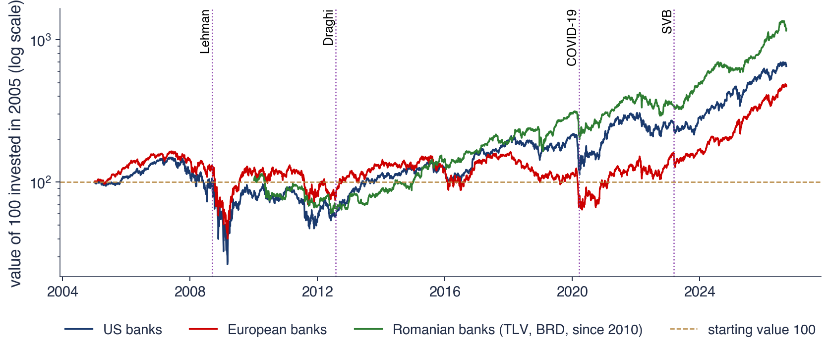

 SFM_ch15_crises