Bucharest University of Economic Studies IDA Institute Digital Assets Blockchain Research Center AI4EFin Artificial Intelligence for Energy Finance Romanian Academy, Institute for Economic Forecasting MSCA Digital Finance
The previous chapters established two facts that seem to contradict each other. Daily S&P 500 returns are almost uncorrelated, so tomorrow's return cannot be anticipated from today's (Chapter 7). Their squares, however, are strongly correlated: the autocorrelation of \(r_t^2\) is 0.31 at lag 1 and still 0.053 at lag 50 (Chapter 8). Large moves follow large moves, of either sign. The daily standard deviation of the index was 0.42% in 2017, but 3.52% between September 2008 and March 2009 and 3.70% between February and May 2020.
This chapter turns the observation into a model. The return is written as an almost constant mean plus a shock whose size, the conditional volatility, depends on the past. The ARCH model of Engle (1982) makes today's variance a function of the squares of recent shocks, and the GARCH(1,1) model of Bollerslev (1986) adds yesterday's variance and obtains, with three parameters, a memory of months. The models are estimated by maximum likelihood, with Normal, Student-t or skewed-t innovations, and extended with the leverage effect (GJR-GARCH, EGARCH).
Applied to six markets, from the S&P 500 to Bitcoin and two stocks of the Bucharest Stock Exchange, the model shows clear differences: equity indices have highly persistent and strongly asymmetric volatility, while Bitcoin has volatility without mean reversion and without a leverage effect. The chapter ends with what makes the model useful in practice: volatility forecasts over several horizons, compared out of sample with EWMA, and a VaR 1% that changes from one day to the next.
Daily log returns of the S&P 500 (%), from January 2000 to 18 September 2026; the shaded bands mark the global financial crisis (September 2008 – March 2009) and the COVID-19 crisis (February – May 2020).
Learning outcomes
Distinguish the conditional from the unconditional variance and explain why returns can be uncorrelated yet dependent.
Write the ARCH(\(q\)) and GARCH(1,1) models and compute the persistence, the unconditional variance and the half-life.
Estimate GARCH models by maximum likelihood, interpret the standard errors and choose the innovation distribution.
Measure the leverage effect with GJR-GARCH, EGARCH and the news impact curve.
Check a fitted model with the standardised residuals and choose between models with AIC and BIC.
Forecast volatility over several horizons, compare forecasts with QLIKE and compute a one-day VaR 1%.
Chapter plan
Volatility ClusteringS&P 500 returns since 2000, two crises and the stylised facts a model must reproduce.
AI for Scientific DiscoveryAn open question on Bitcoin volatility, the help AI can give and the checks it needs.
SummaryKey results, formulas and questions for self-assessment.
Volatility Clustering
The section starts from the data. Daily S&P 500 returns since 2000 alternate calm years and turbulent periods, and two crises, in 2008 and in 2020, show how much and for how long volatility can rise. The section then explains why the conditional variance is a quantity needed by risk management, portfolio choice, derivative pricing and statistical inference, and lists the stylised facts a volatility model must reproduce.
Question for the room Calm days with σ² = 0.5 and stormy days with σ² = 4.5, each with probability 1/2, mean 0. What is the unconditional standard deviation?
Answer
1.58%: the unconditional variance is the average of the variances, 0.5 × 0.5 + 0.5 × 4.5 = 2.50, and √2.50 = 1.58. The average of the volatilities, (0.71 + 2.12)/2 = 1.41%, is smaller, because the square root is concave. The mixture has kurtosis 4.92, although each regime is Normal.
Worked example: unconditional variance, kurtosis and one ARCH(1) step
Question for the room ARCH(1) with ω = 0.5: for α = 0.5 the kurtosis is 9.0. What happens to the kurtosis when ▶ takes α to 0.6?
Answer
It becomes infinite: 3α² = 1.08 ≥ 1, that is α exceeds 1/√3 = 0.577 and the fourth moment no longer exists. The unconditional variance stays finite, ω/(1 − α) = 0.5/0.4 = 1.25.
Question for the room The daily standard deviation of the S&P 500 was 0.42% in 2017. How many times larger was it from September 2008 to March 2009?
Answer
8.3 times: 3.52/0.422 = 8.34; from February to May 2020, 3.70/0.422 = 8.76. The whole-sample standard deviation, 1.21%, averages calm and stormy days and describes neither regime: the 2008 episode is 2.9 times above it.
The chart shows the daily log returns of the S&P 500, \(r_t = 100(\ln P_t - \ln P_{t-1})\), in percent, for 6,714 trading days from January 2000 to 18 September 2026. The largest fall of the sample is −12.8%, on 16 March 2020, and the largest rise is 11.0%, on 13 October 2008. Both extremes fall inside a crisis: the days with the largest gains do not come in good times, but in the same turbulent months as the days with the largest losses.
The dispersion of returns is not constant. The daily standard deviation was 0.42% in 2017, 3.52% between September 2008 and March 2009 and 3.70% between February and May 2020, that is, roughly eight to nine times larger in the crises than in a calm year. On the chart, the two crises, marked with shaded bands, appear as compact blocks of large returns, separated by long years in which returns stay within a few tenths of a percent of zero. A single number for "the volatility of the S&P 500" averages over very different regimes.
The regularity visible on the chart is called volatility clustering: large moves are followed by large moves, of either sign, and small moves by small moves. The sign of tomorrow's return remains unpredictable, but its size does not. Engle (1982) gave the first statistical model of this regularity, and this chapter starts from it.
In brief
Daily log returns \(r_t = 100(\ln P_t - \ln P_{t-1})\), in %, 6 714 days to 18 September 2026; the largest fall: \(-12.8\%\) on 16 March 2020; the largest rise: \(11.0\%\) on 13 October 2008
Standard deviation: \(0.42\%\) in 2017, \(3.52\%\) from September 2008 to March 2009, \(3.70\%\) from February to May 2020
Large changes follow large changes, of either sign: volatility clustering Engle (1982)
The photographs show the two episodes: the Lehman Brothers headquarters in New York on 15 September 2008, the day the bank filed for bankruptcy, and the New York financial district on 25 March 2020, when the COVID-19 pandemic had shut down economies. The causes are very different: a crisis inside the financial system and a shock from outside it.
The effect on volatility was nevertheless similar. The daily standard deviation of the S&P 500 was 8.3 times larger in the financial crisis and 8.8 times larger in the COVID-19 crisis than in 2017. In both cases calm did not return the next day, but only after several months.
The episodes thus show two properties a model must have. Today's variance must depend on recent shocks, so that a turbulent day makes another turbulent day likely. And the effect of a shock must die out slowly, over weeks and months, not in a single day.
In risk management, the value at risk (VaR), the loss exceeded with a given probability, and the expected shortfall (ES), the average loss beyond the VaR, need tomorrow's volatility, not the average volatility of the last 20 years. A VaR computed with a constant variance is too large in calm years and too small in crises, exactly when it matters; Chapter 10 measures this failure with backtesting.
The same need arises elsewhere. The weights of a minimum-variance portfolio depend on variances and covariances that change over time. The price of an option depends on the volatility expected until maturity, and hence on a volatility forecast over a given horizon.
In statistical inference, tests and confidence intervals that assume a constant variance can be wrong when the variance changes: the usual standard errors understate the uncertainty in turbulent periods. This is why Chapter 7 needed random walk tests that remain valid under heteroskedasticity.
In brief
Risk management: VaR (value at risk) and ES (expected shortfall) need tomorrow's volatility, not the average volatility of the last 20 years
a constant-variance VaR is too large in calm years and too small in crises (Chapter 10)
Portfolios: weights depend on variances and covariances, which change over time
Derivatives: option prices depend on the volatility expected until maturity
Inference: tests and confidence intervals that assume a constant variance can be wrong
this is why Chapter 7 needed tests that remain valid under heteroskedasticity
The first fact is volatility clustering, measured by the autocorrelation function (ACF) of squared returns (Chapter 8). For the S&P 500, the autocorrelation of \(r_t^2\) is 0.31 at lag 1 and still 0.053 at lag 50: positive and slowly decaying, the sign of a long memory in the size of returns. The second fact is heavy tails: the kurtosis of daily S&P 500 returns is 13.7, against 3 for the Normal distribution (Chapter 2).
The third fact is the leverage effect: price falls raise volatility more than rises of the same size (Christie, 1982). The fourth is mean reversion of volatility: after a turbulent period volatility does not stay high forever, but returns towards a long-run level. The fifth is the almost complete absence of autocorrelation in returns themselves (Chapter 7).
A volatility model must reproduce all five facts at once: uncorrelated returns with correlated squares, heavy tails, asymmetry and mean reversion. The list serves as a yardstick for the rest of the chapter. GARCH(1,1) explains the clustering, the mean reversion and part of the tails; Student-t innovations explain the rest of the tails; the GJR-GARCH and EGARCH models explain the asymmetry.
In brief
Volatility clustering: the ACF (autocorrelation function) of \(r_t^2\) is positive and decays slowly (Chapter 8)
S&P 500: autocorrelation of \(r_t^2\) at lag 1: \(0.31\); at lag 50: still \(0.053\)
Heavy tails: kurtosis above 3, the value of the Normal distribution (Chapter 2)
S&P 500 daily returns: kurtosis \(13.7\)
Leverage effect: falls raise volatility more than rises of the same size Christie (1982)
Mean reversion of volatility: after a storm, volatility returns to a long-run level
Almost no autocorrelation in \(r_t\) itself (Chapter 7)
Section summary
Daily S&P 500 returns move from a standard deviation of 0.42% in a calm year to more than 3.5% in crises, and turbulent periods last for months. Squared returns are autocorrelated over dozens of lags, returns have a kurtosis of 13.7, and falls raise volatility more than rises. The next section gives a precise meaning to "today's" volatility: the variance conditional on the past.
Conditional Mean and Conditional Variance
The section defines the two conditional quantities the chapter works with, the mean and the variance of the return given past information, and writes the decomposition shared by all models of the chapter. A numerical example shows why the unconditional variance describes no particular day and why a changing variance produces heavy tails.
Let \(\mathcal{F}_{t-1}\) be the information available at the end of day \(t-1\), here the past returns. The conditional mean \(E[X \mid \mathcal{F}_{t-1}]\) is the best forecast of \(X\) given this information, in the mean squared error sense (Chapter 4). For the return, the conditional mean is \(\mu_t = E[r_t \mid \mathcal{F}_{t-1}]\).Chapter 7 showed that for daily returns the past hardly helps to forecast the mean, so \(\mu_t\) can be taken as constant, \(\mu_t = \mu\).
and its square root, \(\sigma_t\), is the conditional volatility. It is known at the end of day \(t-1\), because it depends only on the past, and it changes from one day to the next.
A variance that is not constant is called heteroskedasticity. Conditional heteroskedasticity means something more precise: the variance changes as a function of past information, although the unconditional variance, that of the stationary distribution of returns, can be a constant. The unconditional variance is a single number; the conditional variance is a process, which follows the market from calm periods to turbulent ones.
In brief
\(\mathcal{F}_{t-1}\): the information available at the end of day \(t-1\) (past returns)
conditional expectation \(E[X \mid \mathcal{F}_{t-1}]\): the best forecast of \(X\) given the past (Chapter 4)
The innovations \(z_t\) are i.i.d. with mean 0 and variance 1; their distribution can be Normal, Student-t or another. The shock \(\varepsilon_t\) is the return minus its mean, and the volatility \(\sigma_t\) depends only on the past. The models differ only in the equation that links \(\sigma_t\) to the past and in the distribution of \(z_t\).
Three consequences follow from this form. Since \(\sigma_t\) is known at \(t-1\) and \(z_t\) is independent of the past, \(E[\varepsilon_t \mid \mathcal{F}_{t-1}] = \sigma_t E[z_t] = 0\): the shocks are a martingale difference. By the law of iterated expectations, \(\mathrm{Cov}(\varepsilon_t, \varepsilon_{t-k}) = E[\varepsilon_{t-k} E(\varepsilon_t \mid \mathcal{F}_{t-1})] = 0\), so the shocks are uncorrelated. On the other hand, \(\mathrm{Var}(\varepsilon_t \mid \mathcal{F}_{t-1}) = \sigma_t^2\) is predictable, and \(\varepsilon_t^2\) is correlated with \(\varepsilon_{t-1}^2\), because \(\sigma_t\) depends on past shocks. The shocks are uncorrelated, but not independent.
In the terms of Chapter 7, the RW1 hypothesis, with i.i.d. increments, is rejected, while the RW3 hypothesis, with uncorrelated increments, still holds. The decomposition reconciles the two facts from the start of the chapter: a market in which the return cannot be predicted can have a predictable risk.
In brief
Every model of this chapter has the form \(r_t = \mu + \varepsilon_t\), \(\varepsilon_t = \sigma_t z_t\)
\(z_t\): the innovations, i.i.d. with mean 0 and variance 1 (Normal, Student-t, …)
\(\varepsilon_t\): the shock (the return minus its mean); \(\sigma_t\) depends only on the past
Consequences
\(E[\varepsilon_t \mid \mathcal{F}_{t-1}] = \sigma_t E[z_t] = 0\): the shocks are a martingale difference, hence uncorrelated
\(\mathrm{Var}(\varepsilon_t \mid \mathcal{F}_{t-1}) = \sigma_t^2\): the variance is predictable
the \(\varepsilon_t\) are uncorrelated but not independent: \(\varepsilon_t^2\) is correlated with \(\varepsilon_{t-1}^2\)
In the terms of Chapter 7: RW1 (i.i.d. increments) is rejected, RW3 (uncorrelated increments) is kept
Worked Example: Conditional and Unconditional Variance
Consider a market with two kinds of days: calm days, with conditional variance \(\sigma_t^2 = 0.5\), and turbulent days, with \(\sigma_t^2 = 4.5\), each with probability \(1/2\), and a conditional mean of 0. The law of total variance splits the unconditional variance into the mean of the conditional variances plus the variance of the conditional means:
Step by step, \(\mathrm{Var}(r_t) = 0.5 \times 0.5 + 0.5 \times 4.5 + 0 = 2.50\), so the unconditional standard deviation is \(\sqrt{2.50} = 1.58\%\). On a calm day, however, \(\sigma_t = 0.71\%\), and on a turbulent day \(\sigma_t = 2.12\%\). The average of 1.58% describes neither day: the unconditional variance is an average, while the conditional variance tells us what kind of day we are in.
The example also shows where heavy tails come from. If \(z_t\) is Normal, \(r_t\) is a mixture of Normal distributions with different variances, and \(E[r_t^4] = 3E[\sigma_t^4]\). The kurtosis is then \(3E[\sigma_t^4]/(E[\sigma_t^2])^2\), which exceeds 3 whenever \(\sigma_t\) varies, by Jensen's inequality. In the example, \(E[\sigma_t^4] = (0.25 + 20.25)/2 = 10.25\), and the kurtosis is \(3 \times 10.25/6.25 = 4.92\). Conditional heteroskedasticity creates kurtosis even with Normal innovations.
In brief
A market has calm days (\(\sigma_t^2 = 0.5\)) and stormy days (\(\sigma_t^2 = 4.5\)), each with probability \(1/2\); the mean is 0
law of total variance: \(\mathrm{Var}(r_t) = E[\mathrm{Var}(r_t \mid \mathcal{F}_{t-1})] + \mathrm{Var}(E[r_t \mid \mathcal{F}_{t-1}])\)
step by step: \(0.5 \times 0.5 + 0.5 \times 4.5 + 0 = 2.50\), so the unconditional standard deviation is \(1.58\%\)
The unconditional variance is an average; the conditional variance tells which day we are in
a calm day: \(\sigma_t = 0.71\%\); a stormy day: \(\sigma_t = 2.12\%\); the average \(1.58\%\) fits neither
A mixture of Normal distributions with different variances has heavy tails: conditional heteroskedasticity creates kurtosis
Section summary
The conditional mean of daily returns is almost constant, while the conditional variance \(\sigma_t^2\) changes from day to day. The decomposition (9.1) produces shocks that are uncorrelated but dependent, and the mixture of calm and turbulent days produces heavy tails. The next section presents the first model for \(\sigma_t^2\), the ARCH model.
The ARCH Model
The ARCH model makes today's variance a linear function of the squares of recent shocks. The section presents its origin, the definition and properties of the ARCH(1) model, a comparison of simulated paths, and the ARCH(\(q\)) extension together with its main limitation: to reproduce the long memory of volatility, the model needs many lags.
Engle (1982) introduced the ARCH model (autoregressive conditional heteroskedasticity), in which today's variance depends on the squares of yesterday's shocks. The first application was not to financial markets but to the variance of United Kingdom inflation; the paper was written during Engle's visit to the London School of Economics.
The contribution was recognised by the 2003 Nobel Prize in economics, "for methods of analyzing economic time series with time-varying volatility (ARCH)", shared with Clive Granger, honoured for cointegration. Engle's Nobel lecture (Engle, 2004) describes the path from the original model to its use in risk management. The photographs show Robert F. Engle in 2022 and the Stockholm Concert Hall, where the Nobel Prizes are awarded.
The idea changed the status of the variance in econometrics. Before, the variance was treated as a constant or estimated on rolling windows, without a model of its dynamics. ARCH turned the conditional variance into a parametric object, which is estimated by maximum likelihood, tested and forecast.
with \(\omega > 0\) and \(\alpha \ge 0\). In words, today's variance is a constant plus a fraction \(\alpha\) of the square of yesterday's shock. The parameter \(\omega\) is the variance after a zero shock, and \(\alpha\) measures the reaction to yesterday's shock; the restrictions ensure a positive variance. Because the shock enters squared, a large shock yesterday, positive or negative, raises today's variance.
The name "autoregressive" comes from a rewriting. Let \(v_t = \varepsilon_t^2 - \sigma_t^2 = \sigma_t^2(z_t^2 - 1)\), the surprise in the squared shock; \(E[v_t \mid \mathcal{F}_{t-1}] = 0\), because \(E[z_t^2] = 1\). Substituting \(\sigma_t^2 = \varepsilon_t^2 - v_t\) in the variance equation gives \(\varepsilon_t^2 = \omega + \alpha\,\varepsilon_{t-1}^2 + v_t\): the squared shocks follow an AR(1) model, with an error \(v_t\) that is a martingale difference, but heteroskedastic.
The dynamics of the squares follow. When the fourth moment exists, the ACF of \(\varepsilon_t^2\) is \(\rho(k) = \alpha^k\), as for any AR(1). The model therefore produces volatility clustering, but the autocorrelation decays geometrically at rate \(\alpha\): for \(\alpha = 0.5\) it is already \(0.5^5 \approx 0.03\) at lag 5, whereas for the S&P 500 the autocorrelation of \(r_t^2\) is still 0.053 at lag 50.
ARCH(1) shocks have mean zero and are uncorrelated, \(\mathrm{Cov}(\varepsilon_t, \varepsilon_{t-k}) = 0\) for \(k \ne 0\), like any martingale difference. The unconditional variance follows by taking the mean of the variance equation. If the process is stationary, \(\bar\sigma^2 = E[\varepsilon_t^2] = E[\sigma_t^2] = \omega + \alpha\bar\sigma^2\), so \(\bar\sigma^2 = \omega/(1 - \alpha)\), a finite and positive quantity only for \(\alpha < 1\).
With Normal innovations and \(3\alpha^2 < 1\), the kurtosis of the shocks is
The innovations are Normal, yet the returns are heavy-tailed (Franke, Härdle & Hafner, 2019), for the reason of the example in the previous section: \(\varepsilon_t\) is a mixture of Normal distributions with random variances. If \(\alpha \ge 1/\sqrt{3} = 0.577\), the fourth moment is infinite, although the variance remains finite for \(\alpha < 1\).
The worked example uses \(\omega = 0.5\) and \(\alpha = 0.5\). The unconditional variance is \(\bar\sigma^2 = 0.5/0.5 = 1.00\), and the kurtosis is \(K = 3 \times 0.75/0.25 = 9.0\). After a shock \(\varepsilon_{t-1} = 2\), two unconditional standard deviations, today's variance is \(\sigma_t^2 = 0.5 + 0.5 \times 4 = 2.50\), and \(\sigma_t = 1.58\): a single two-standard-deviation shock lifts today's variance to 2.5 times its unconditional level.
In brief
Mean and autocorrelation: \(E[\varepsilon_t] = 0\), \(\mathrm{Cov}(\varepsilon_t, \varepsilon_{t-k}) = 0\) for \(k \ne 0\)
Unconditional variance (if \(\alpha < 1\)): take expectations in \(\sigma_t^2 = \omega + \alpha\varepsilon_{t-1}^2\)
Models with Normal innovations (in green: the smallest AIC and BIC)
Question for the room S&P 500: ARCH(10) has 12 parameters and log-likelihood −9,227.6; GARCH(1,1) has 4 parameters and −9,218.0. Which model does BIC prefer?
Answer
GARCH(1,1): BIC 18,471.2 against 18,561.0 for ARCH(10), 89.8 lower. It has a higher likelihood with a third of the parameters: the term βσ²(t − 1) summarises all past shocks with geometric weights. The BIC of ARCH(q) falls with every added lag up to q = 10, but stays above that of GARCH(1,1).
Worked example: long-run variance and kurtosis
\[\bar\sigma^2 = \frac{\omega}{1-\alpha-\beta}, \qquad K = 3\,\frac{1-(\alpha+\beta)^2}{1-(\alpha+\beta)^2-2\alpha^2}\]
Question for the room α = 0.10 and β = 0.88 give kurtosis 6.06. What does the kurtosis become when ▶ takes β to 0.89?
Answer
Infinite: (α + β)² + 2α² = 0.9801 + 0.02 = 1.0001 ≥ 1. The unconditional variance stays finite (α + β = 0.99 < 1; with ω = 0.02, σ̄² = 2.00), but the fourth moment no longer exists: the condition for the kurtosis is stricter than that for stationarity.
Question for the room For α + β = 0.98 the half-life is 34.3 days. What is it for α + β = 0.99?
Answer
69.0 days, almost double: h½ ≈ ln 2/(1 − α − β), and 1 − α − β halves, from 0.02 to 0.01. For 0.90 it is 6.6 days; for the S&P 500 (α + β = 0.9947), 131 days.
Question for the room With σ²(t) = 1.2 and r(t) = −3%, σ²(t + 1) = 1.976. What is σ²(t + 1) after r(t) = +3%?
Answer
Also 1.976: GARCH(1,1) uses ε², so the sign of the shock does not matter (here μ = 0). The value 1.376 = 0.02 + 0.10 × 3 + 0.88 × 1.2 forgets the square. Asymmetry needs GJR-GARCH or EGARCH (Section 8).
Worked example: IGARCH and GARCH forecasts after a crash
Question for the room An analyst forecasts the volatility one year ahead with EWMA right after a crash. What goes wrong?
Answer
EWMA keeps the crisis level for the whole year. S&P 500, at the close of 16 March 2020: EWMA (λ = 0.94) forecasts 84.0% a year for every horizon; GARCH(1,1)-t starts at 111.0% and falls to 62.0% after 250 days, towards the long-run level of 27.3%. EWMA is an IGARCH with ω = 0: no mean reversion.
Question for the room For ARCH(1) with ω = α = 0.5 the theoretical kurtosis is 9.0. What kurtosis does the simulated series of 1000 values have?
Answer
4.91, far below 9.0: the fourth moment converges slowly, because it depends on a few rare spikes. The i.i.d. series has 3.12 (theory 3), GARCH(1,1) has 3.74 (theory 6.06). With other seeds of the generator the sample values change a lot.
The chart compares three simulated series of 1000 values each, all with unconditional variance 1: an i.i.d. Normal series, an ARCH(1) with \(\omega = \alpha = 0.5\) and a GARCH(1,1) with \(\omega = 0.02\),\(\alpha = 0.10\) and \(\beta = 0.88\), the model of the next section. Since the unconditional variance is the same, the differences between the panels come only from the dynamics of the variance.
The sample kurtosis is 3.12 for the i.i.d. series, 4.91 for ARCH and 3.74 for GARCH, against theoretical values of 3, 9.0 and 6.06. The gap between sample and theoretical values shows that the fourth moment converges slowly: it depends on a few very large values, and 1000 observations contain few of them. The same makes the sample kurtosis of real returns an unstable quantity.
The panels show the difference in dynamics. ARCH(1) produces isolated spikes: its memory is one day, so a large shock raises the next day's variance and the effect disappears quickly. GARCH(1,1) produces long calm periods and long turbulent periods, as around values 250 and 850, like the actual S&P 500 returns in the first chart of the chapter.
In brief
Three series of 1000 values with unconditional variance 1; ARCH(1) with \(\omega = \alpha = 0.5\), GARCH(1,1) with \(\omega = 0.02\), \(\alpha = 0.10\), \(\beta = 0.88\) (next section)
Sample kurtosis: i.i.d. \(3.12\), ARCH \(4.91\), GARCH \(3.74\); theory: 3, \(9.0\), \(6.06\); the fourth moment converges slowly
ARCH(1) gives isolated spikes; GARCH(1,1) gives long calm and long agitated periods, as in real returns
The ARCH(\(q\)) model includes \(q\) lags: \(\sigma_t^2 = \omega + \alpha_1\varepsilon_{t-1}^2 + \dots + \alpha_q\varepsilon_{t-q}^2\), with \(\alpha_i \ge 0\), stationary if \(\sum_i \alpha_i < 1\). The coefficient \(\alpha_i\) measures the reaction to the shock of \(i\) days ago. The effect of a shock lasts exactly \(q\) days, whereas volatility clustering in real data lasts months; to reproduce it, \(q\) must be large, with many parameters constrained to be non-negative.
The presence of ARCH effects is tested with Engle's Lagrange multiplier test (ARCH-LM): the regression of \(\hat\varepsilon_t^2\) on its own \(q\) lags, with the statistic \(TR^2\), which has a \(\chi^2(q)\) distribution if there are no ARCH effects (Chapter 8). A rejection shows that the squared residuals are predictable from their past.
The table estimates ARCH(1), ARCH(5), ARCH(10) and GARCH(1,1) on the S&P 500 with Normal innovations. The log-likelihood rises from −10,305.5 for ARCH(1), with 3 parameters, to −9,340.5 for ARCH(5), with 7 parameters, and to −9,227.6 for ARCH(10), with 12 parameters, while the sum of the coefficients \(\alpha_i\) rises from 0.394 to 0.816 and to 0.849. GARCH(1,1), with only 4 parameters, has a higher log-likelihood (−9,218.0), persistence \(\alpha + \beta = 0.980\) and the smallest information criteria: AIC 18,444.0 and BIC 18,471.2, against 18,479.3 and 18,561.0 for ARCH(10). The AIC and BIC criteria, for which a smaller value is better, are defined in Section 10. ARCH needs ten lags and still falls short of a four-parameter model; the missing ingredient is long memory.
ARCH(1) makes today's variance a function of the square of yesterday's shock, (9.2). The model produces uncorrelated shocks, the unconditional variance \(\omega/(1 - \alpha)\) and heavy tails even with Normal innovations, but its memory is short. ARCH(\(q\)) lengthens the memory at the price of many parameters, and on the S&P 500 even ARCH(10) does not reach the likelihood of a four-parameter GARCH(1,1). The next section presents this model.
The GARCH(1,1) Model
GARCH(1,1) adds yesterday's variance to the variance equation and thus obtains, with three parameters, an ARCH with infinitely many lags and geometric weights. The section defines the model, derives the stationarity condition, the long-run variance and the kurtosis, introduces persistence and the half-life, applies them in an example and shows the link with IGARCH and EWMA.
Bollerslev (1986), then Engle's doctoral student at the University of California, San Diego, added yesterday's variance to the variance equation. The GARCH model (generalised ARCH) replaces a long ARCH(\(q\)) with a few parameters. The photograph shows the university's Geisel Library.
A year later, Bollerslev (1987) combined the model with Student-t innovations to describe the heavy tails of returns, the combination used in Section 6 of this chapter.
GARCH(1,1) has remained the benchmark. Hansen & Lunde (2005) compared 330 volatility models and found none that beat it on exchange rates; for the returns of a stock, models that include the leverage effect did better. Both results reappear on the data of this chapter, in the sections on asymmetry and on forecasting.
In brief
Bollerslev (1986), a doctoral student of Engle at the University of California, San Diego: add yesterday's variance to the equation
GARCH (generalised ARCH): a few parameters replace a long ARCH(\(q\))
with \(\omega > 0\),\(\alpha \ge 0\) and \(\beta \ge 0\), restrictions that keep the variance positive. Each parameter has a role. \(\alpha\) is the reaction to yesterday's news, the size of the jump in variance after a shock. \(\beta\) is the memory of the variance, the part of yesterday's level that is kept today. The sum \(\alpha + \beta\) is the persistence, and \(\omega\) fixes, together with it, the long-run level.
Substituting \(\sigma_{t-1}^2\),\(\sigma_{t-2}^2\), … repeatedly in the equation gives
GARCH(1,1) is thus an ARCH(\(\infty\)) with geometric weights: all past shocks matter, and the shock of \(j + 1\) days ago receives the weight \(\alpha\beta^j\). With \(\beta\) close to 1 the weights decay slowly, and three parameters produce the memory of months that ARCH(\(q\)) obtained only with dozens of lags.
The shape of the weights is the same as that of the exponentially weighted moving average of Chapter 8. The difference is the constant \(\omega/(1 - \beta)\), which pulls the variance towards a long-run level; the exact link with EWMA comes at the end of the section.
As for ARCH, let \(v_t = \varepsilon_t^2 - \sigma_t^2\) be the surprise in the squared shock. Substituting in (9.3) gives \(\varepsilon_t^2 = \omega + (\alpha + \beta)\varepsilon_{t-1}^2 + v_t - \beta v_{t-1}\): the squared shocks follow an ARMA(1,1) model (autoregressive moving average). The autoregressive part has coefficient \(\alpha + \beta\), so the ACF of \(\varepsilon_t^2\) decays like \((\alpha + \beta)^k\) at lag \(k\). With a small \(\alpha\) and \(\alpha + \beta\) close to 1, the autocorrelations of the squares are moderate but decay very slowly, as for the S&P 500.
The process is covariance stationary if \(\alpha + \beta < 1\). Then the unconditional variance, also called the long-run variance, is
and the corresponding annualised volatility is \(\sqrt{252\,\bar\sigma^2}\), with 252 trading days per year. The denominator \(1 - \alpha - \beta\) is small when the persistence is close to 1, which makes \(\bar\sigma^2\) sensitive to small errors in the parameters.
With Normal innovations and \((\alpha + \beta)^2 + 2\alpha^2 < 1\), the kurtosis of the shocks is
For \(\alpha = 0.10\) and \(\beta = 0.88\),\((\alpha + \beta)^2 + 2\alpha^2 = 0.9804\) and \(K = 6.06\). The condition for a finite fourth moment is close to its limit: a slightly larger \(\alpha\), at the same persistence, makes the kurtosis infinite.
In brief
As for ARCH: \(\varepsilon_t^2 = \omega + (\alpha + \beta)\varepsilon_{t-1}^2 + v_t - \beta v_{t-1}\), an ARMA(1,1) for the squared shocks
\(v_t = \varepsilon_t^2 - \sigma_t^2\): the surprise in the squared shock, as for ARCH(1)
ARMA: autoregressive moving average; the ACF of \(\varepsilon_t^2\) decays like \((\alpha + \beta)^k\) at lag \(k\)
Covariance stationary if \(\alpha + \beta < 1\); then the unconditional (long-run) variance is
\(\bar\sigma^2 = E[\sigma_t^2] = \dfrac{\omega}{1 - \alpha - \beta}\), annualised volatility \(\sqrt{252\,\bar\sigma^2}\) for 252 trading days
Kurtosis with Normal \(z_t\), if \((\alpha + \beta)^2 + 2\alpha^2 < 1\): \(K = 3\,\dfrac{1 - (\alpha + \beta)^2}{1 - (\alpha + \beta)^2 - 2\alpha^2} > 3\)
where \(E[\cdot \mid \mathcal{F}_t]\) is the forecast made at the end of day \(t\) and \(\bar\sigma^2\) is the long-run variance. The deviation of the variance from its long-run level shrinks by the factor \(\alpha + \beta\) every day. The persistence therefore says how fast the model forgets a shock.
The half-life is the number of days after which half of a variance shock has gone. From \((\alpha + \beta)^h = 1/2\),
For \(\alpha + \beta = 0.90\), the half-life is 6.6 days; for 0.98 it is 34.3 days; for 0.99 it is 69.0 days. Small changes in persistence near 1 matter a great deal: moving from 0.98 to 0.99 doubles the half-life.
For daily stock returns, typical estimates are \(\alpha\) around 0.05–0.15 and \(\beta\) around 0.80–0.93, with \(\alpha + \beta\) close to 1. The reaction to one day's news is small and the memory is long; Section 7 confirms this pattern in six markets.
In brief
Forecast of the variance \(h\) days ahead (derived in Section 11): \(E[\sigma_{t+h}^2 \mid \mathcal{F}_t] - \bar\sigma^2 = (\alpha + \beta)^{h-1}(\sigma_{t+1}^2 - \bar\sigma^2)\)
\(E[\cdot \mid \mathcal{F}_t]\): the forecast made at the end of day \(t\); \(\bar\sigma^2\): the long-run variance
a deviation from the long-run variance shrinks by the factor \(\alpha + \beta\) each day
Half-life: the number of days after which half of a variance shock is gone
For daily returns in percent, take \(\omega = 0.02\),\(\alpha = 0.10\),\(\beta = 0.88\) and \(\mu = 0\). The persistence is \(\alpha + \beta = 0.98\), the long-run variance is \(\bar\sigma^2 = 0.02/(1 - 0.98) = 1.00\), so the long-run annualised volatility is \(\sqrt{252 \times 1.00} = 15.9\%\). The half-life is \(\ln 0.5/\ln 0.98 = 34.3\) days.
Today the conditional variance is \(\sigma_t^2 = 1.2\) and the return is \(r_t = -3\%\), so the shock is \(\varepsilon_t = -3\). Tomorrow's variance is \(\sigma_{t+1}^2 = 0.02 + 0.10 \times 9 + 0.88 \times 1.2 = 1.976\), and tomorrow's volatility is \(\sigma_{t+1} = 1.41\%\). The three terms show the contributions: 0.02 from the constant, 0.90 from today's shock and 1.056 from the memory of today's variance.
The shock has raised the variance from 1.2 to almost 2. Without new shocks, it then declines towards 1.00 by the factor 0.98 per day, and the excess of 0.976 over the long-run level halves in about 34 days. A return of +3% would have produced exactly the same variance: GARCH(1,1) does not distinguish between signs.
The IGARCH model (integrated GARCH) (Engle & Bollerslev, 1986) is the limiting case \(\alpha + \beta = 1\). Variance shocks no longer die out: the shrinking factor in (9.5) is 1, so there is no half-life and no finite unconditional variance. The variance forecast no longer reverts to a long-run level: with \(\omega = 0\) it is the same for every horizon, and with \(\omega > 0\) it grows linearly with the horizon, \(E_t[\sigma_{t+h}^2] = \sigma_{t+1}^2 + (h - 1)\omega\).
The exponentially weighted moving average (EWMA) of Chapter 8, \(\sigma_t^2 = \lambda\sigma_{t-1}^2 + (1 - \lambda)r_{t-1}^2\), is an IGARCH with \(\omega = 0\),\(\alpha = 1 - \lambda\) and \(\beta = \lambda\). The RiskMetrics methodology uses \(\lambda = 0.94\) for daily data. The two methods have opposite advantages: EWMA has nothing to estimate but no mean reversion; GARCH has three parameters to estimate, and its volatility reverts to \(\bar\sigma\).
Question for the class: an analyst forecasts next year's volatility with EWMA right after a crash. Where does the analyst go wrong? Answer: EWMA keeps today's crisis level for the whole year, while GARCH lets it decline towards the long-run level, at the speed set by the persistence. Over a long horizon, the gap between the two forecasts is large precisely after a large shock.
this is IGARCH with \(\omega = 0\), \(\alpha = 1 - \lambda\), \(\beta = \lambda\); RiskMetrics uses \(\lambda = 0.94\) for daily data
EWMA: nothing to estimate, but no mean reversion; GARCH: three parameters, and volatility returns to \(\bar\sigma\)
Question for the room: an analyst forecasts the volatility one year ahead with EWMA right after a crash. What goes wrong?
Answer: EWMA keeps today's crisis level for the whole year; GARCH lets it decay towards the long-run level
Section summary
GARCH(1,1), (9.3), is an ARCH(\(\infty\)) with geometric weights. For \(\alpha + \beta < 1\) the process is stationary, with the long-run variance (9.4), and forecasts revert towards it by the factor \(\alpha + \beta\) per day; the half-life (9.6) turns the persistence into days. IGARCH and EWMA are the limiting case without mean reversion. The next section shows how the parameters are estimated.
Estimation by Maximum Likelihood
The parameters of a GARCH model are estimated by maximum likelihood. The section writes the conditional log-likelihood, shows on simulated data how its shape changes with the sample size, estimates GARCH(1,1) for the S&P 500 with a direct implementation and with a dedicated package, and explains why the standard errors must be computed robustly when the innovations are not Normal.
The returns of a GARCH model are dependent, so their joint density is not a product of marginal densities. It does, however, factor into conditional densities: with \(f\) a density, \(T\) the number of returns and \(\theta\) the parameter vector, \(f(r_1, \dots, r_T) = f(r_1)\prod_{t=2}^{T} f(r_t \mid \mathcal{F}_{t-1})\). With Normal innovations, each factor is a Normal density, \(r_t \mid \mathcal{F}_{t-1} \sim N(\mu, \sigma_t^2)\).
Conditioning on the first observation and taking logs, the conditional log-likelihood for \(\theta = (\mu, \omega, \alpha, \beta)\) is
Each day adds two penalties: one for a large \(\sigma_t^2\) and one for a large squared error relative to \(\sigma_t^2\). The first pushes the variance down, the second up, and the maximum balances the two. The variances \(\sigma_t^2(\theta)\) are computed recursively with (9.3), starting from an initial value \(\sigma_1^2\), for example the sample variance.
The maximum likelihood estimator (MLE) is \(\hat\theta = \arg\max_\theta \ell(\theta)\), subject to \(\omega > 0\),\(\alpha, \beta \ge 0\) and \(\alpha + \beta < 1\). Because \(\sigma_t^2(\theta)\) depends on the parameters through a recursion, there is no closed-form formula for \(\hat\theta\); a numerical optimisation algorithm searches for the maximum (Franke, Härdle & Hafner, 2019).
In brief
The returns are dependent, so we factor the joint density into conditional densities
\(f\): a probability density; \(T\): the number of returns; \(\theta\): the vector of parameters; \(\ell\): the log-likelihood
\(f(r_1, \dots, r_T) = f(r_1)\prod_{t=2}^{T} f(r_t \mid \mathcal{F}_{t-1})\), and \(r_t \mid \mathcal{F}_{t-1} \sim N(\mu, \sigma_t^2)\) for Normal innovations
Conditional log-likelihood with \(\theta = (\mu, \omega, \alpha, \beta)\):
Question for the room With n = 100, α̂ = 0.432 and the standard error is 0.127. How does the standard error change with n = 1000?
Answer
It falls to 0.035, 3.6 times smaller; the √n rule gives √10 = 3.16. The log-likelihood curve gets sharper, and α̂ = 0.491 is closer to the true value 0.5.
The chart shows the log-likelihood of a simulated ARCH(1) with \(\omega = \alpha = 0.5\), as a function of \(\alpha\), with \(\omega = 1 - \alpha\), so that the unconditional variance stays at 1. Each curve is drawn minus its maximum, so its peak is at zero, and the vertical axis measures how much the likelihood loses as \(\alpha\) moves away from the estimate.
With \(n = 100\) observations, the maximum is at \(\hat\alpha = 0.432\), with standard error 0.127; with \(n = 1000\), the maximum is at \(\hat\alpha = 0.491\), with standard error 0.035, close to the true value 0.5. The ratio of the standard errors, \(0.127/0.035 \approx 3.6\), is of the order of \(\sqrt{10} = 3.16\), as the \(1/\sqrt{n}\) rate predicts.
The geometric interpretation is direct. The curve for \(n = 100\) is almost flat over a wide range of values of \(\alpha\): the data do not distinguish these values well. The curve for \(n = 1000\) is much sharper. The curvature of the log-likelihood at its maximum, the observed Fisher information, gives the standard error: a large curvature means a small standard error.
In brief
Simulated ARCH(1) with \(\omega = \alpha = 0.5\); \(\ell(\alpha)\) with \(\omega = 1 - \alpha\), as in SFElikarch1; each curve minus its maximum
GARCH(1,1) with Normal innovations: step by step (scipy) and with the arch package
Question for the room S&P 500, GARCH(1,1) with Normal innovations: the classic SE of α̂ is 0.0086. What is the robust SE?
Answer
0.0118, 1.37 times larger (β: 1.37; ω: 1.63; μ: 1.02). The innovations have heavy tails, and the classic SE, computed as if z(t) were Normal, overstate the precision of the variance parameters. For the BET the ratio exceeds 2.6.
GARCH(1,1) with three innovation distributions
Question for the room Moving from Normal to Student-t innovations raises the S&P 500 log-likelihood from −9,218.0 to −9,062.5. Do α and β change much?
Answer
Little: α from 0.121 to 0.123, β from 0.860 to 0.872; the persistence rises from 0.980 to 0.995. The LR statistic, 311.0, is far above 3.84: the innovation distribution matters for the tail quantiles (VaR) more than for σ(t).
Question for the room With n = 500 the maximum on the grid is at (0.045, 0.63), far from the true values (0.1, 0.8). Where is the maximum with n = 2000?
Answer
At (0.100, 0.78), close to the true values: the long ridge along which α and β trade off narrows as n grows. With other seeds of the generator (extra runs) the maximum for n = 500 ranges from (0.025, 0.95) to (0.205, 0.67).
The chart shows the contours of the log-likelihood of a simulated GARCH(1,1) with \(\omega = 0.1\),\(\alpha = 0.1\) and \(\beta = 0.8\), as a function of \((\alpha, \beta)\), minus its maximum. The constant \(\omega\) is set so that the unconditional variance of the model equals the sample variance, which reduces the problem to two parameters. The dashed line marks the IGARCH boundary, \(\alpha + \beta = 1\).
With \(n = 500\) observations, the maximum on the grid is at \(\alpha = 0.045\) and \(\beta = 0.63\), far from the true values, and the contours do not close around it: the likelihood falls very little along an entire direction. With \(n = 2000\), the maximum is at \(\alpha = 0.10\) and \(\beta = 0.78\), and the contours become closed ellipses around the true values.
The shape of the contours has an explanation. Along a long, flat ridge, \(\alpha\) and \(\beta\) offset each other: a smaller \(\alpha\) and a different \(\beta\) can produce variance paths that are almost equally plausible. The errors of the two estimates are therefore strongly negatively correlated, and GARCH needs long samples, of the order of thousands of daily observations, to be estimated precisely.
In brief
Simulated GARCH(1,1), \(\omega = 0.1\), \(\alpha = 0.1\), \(\beta = 0.8\); \(\omega\) set so that the unconditional variance equals the sample variance, as in SFElikgarch; contours: log-likelihood minus its maximum
\(n = 500\): maximum at \((0.045, 0.63)\), far from the truth; \(n = 2000\): \((0.100, 0.78)\)
Interpretation: a long, flat ridge along which \(\alpha\) and \(\beta\) trade off: GARCH needs long samples
The table estimates GARCH(1,1) with Normal innovations for the S&P 500 in two ways: with a direct implementation, which writes \(-\ell(\theta)\) from (9.7) and minimises it numerically under the restriction \(\alpha + \beta < 1\), and with the Python package arch. The estimates agree to the third significant digit: \(\mu\) is 0.0614 against 0.0615, \(\omega\) 0.0253 against 0.0254, \(\alpha\) 0.1205 against 0.1206 and \(\beta\) 0.8600 against 0.8599. The two versions differ only in the initial value of \(\sigma_t^2\) and in the optimisation algorithm, which also explains the small difference in the maximised log-likelihood, −9,219.9 against −9,218.0.
Standard errors (SE) can be computed in two ways. The classical standard error comes from the inverse of the Hessian matrix, the curvature of \(\ell\) at its maximum, and assumes that the innovations really are Normal. The robust standard error (Bollerslev & Wooldridge, 1992) remains valid when \(z_t\) is not Normal. For the S&P 500, the classical errors are 0.0098 for \(\mu\), 0.0030 for \(\omega\), 0.0086 for \(\alpha\) and 0.0091 for \(\beta\), and the robust ones are 0.0100, 0.0048, 0.0118 and 0.0125.
The robust standard errors of the variance parameters are larger: about 1.4 times for \(\alpha\) and \(\beta\) and 1.6 times for \(\omega\), while for \(\mu\) the two errors almost coincide. When \(z_t\) has heavy tails, the classical errors overstate the precision of the variance-equation estimates, and the confidence intervals built from them are too narrow.
In brief
S&P 500, GARCH(1,1)-N
step by step (SE)
arch
classic SE
robust SE
\(\mu\)
\(0.0614\) (\(0.0098\))
\(0.0615\)
\(0.0098\)
\(0.0100\)
\(\omega\)
\(0.0253\) (\(0.0030\))
\(0.0254\)
\(0.0030\)
\(0.0048\)
\(\alpha\)
\(0.1205\) (\(0.0086\))
\(0.1206\)
\(0.0086\)
\(0.0118\)
\(\beta\)
\(0.8600\) (\(0.0091\))
\(0.8599\)
\(0.0091\)
\(0.0125\)
Step by step: write \(-\ell(\theta)\) in Python and minimise it with scipy.optimize.minimize under \(\alpha + \beta < 1\)
the two routes differ only in the start-up of \(\sigma_t^2\) and in the optimiser; log-likelihood \(-9219.9\) against \(-9218.0\)
SE (standard error), classic: from the inverse Hessian (the curvature of \(\ell\)); robust: valid when \(z_t\) is not Normal Bollerslev & Wooldridge (1992)
Interpretation: the robust SE of \(\alpha\) and \(\beta\) are about 1.4 times larger (1.6 for \(\omega\), 1.02 for \(\mu\)): with heavy-tailed \(z_t\) the classic SE overstate the precision of the variance parameters
Quasi-maximum likelihood estimation (QMLE) maximises the Normal likelihood (9.7) even if \(z_t\) is not Normal. Bollerslev & Wooldridge (1992) showed that the estimates remain consistent if the mean \(\mu\) and the conditional variance \(\sigma_t^2\) are correctly specified. The reason is that the derivatives of the Normal log-likelihood have mean zero whenever the first two conditional moments are right, whatever the rest of the distribution.
The classical standard errors are wrong, however, because the equality between the Hessian and the variance of the derivatives, which holds when the assumed distribution is the true one, no longer holds. The robust "sandwich" standard error combines the two matrices, \(A^{-1}BA^{-1}\), where \(A\) is the Hessian and \(B\) is the variance of the log-likelihood derivatives. When the innovations are Normal, \(A\) and \(B\) coincide and the formula reduces to the classical one.
Several practical rules follow. Report the robust standard errors, which are the default in the arch package. Use at least 1000–2000 daily observations, and express returns in percent, to avoid numerical problems caused by a very small \(\omega\). An estimate on the boundary, with \(\alpha + \beta = 1\), has no ordinary standard error and is reported as IGARCH. QMLE is consistent but not efficient: a better-fitting innovation distribution gives more precise estimates, the subject of the next section.
In brief
QMLE (quasi-maximum likelihood estimation): maximise the Normal likelihood even if \(z_t\) is not Normal
but the classic SE are wrong: use the robust (“sandwich”) SE
Practical rules
report robust SE (the default of arch)
use at least 1000–2000 daily observations; returns in % avoid numerical problems with tiny \(\omega\)
an estimate on the boundary (\(\alpha + \beta = 1\)) has no usual standard error: report it as IGARCH
A better innovation distribution gives more efficient estimates: next section
Section summary
The GARCH log-likelihood, (9.7), is maximised numerically, with the variances computed recursively. On simulated data it is flat in small samples and has a ridge along which \(\alpha\) and \(\beta\) offset each other, which is why GARCH needs long samples. On the S&P 500, the direct implementation and the package give the same estimates, and the robust standard errors of the variance parameters are 1.4–1.6 times the classical ones. The next section replaces the Normal innovations with heavy-tailed distributions.
Heavy-Tailed Innovations
GARCH with Normal innovations explains only part of the kurtosis of returns. The section introduces Student-t and skewed-t innovations, compares them on the S&P 500 with likelihood ratio tests and checks the fit of the tails with QQ plots of the standardised residuals.
A GARCH with Normal innovations explains part of the heavy tails through the variation of \(\sigma_t\), but not all of them. S&P 500 returns have a kurtosis of 13.7, while the standardised residuals \(\hat z_t = \hat\varepsilon_t/\hat\sigma_t\) of a Normal GARCH(1,1) have a kurtosis of 4.7. If the variance model is correct, the remaining heavy tails must come from the distribution of \(z_t\).
The first choice is the standardised Student-t distribution with \(\nu > 2\) degrees of freedom (Bollerslev, 1987), from Chapter 2. If \(t_\nu\) is a Student-t variable with \(\nu\) degrees of freedom, \(z_t = t_\nu\sqrt{(\nu - 2)/\nu}\) has variance 1, as (9.1) requires. A small \(\nu\) means heavy tails: the kurtosis is \(3 + 6/(\nu - 4)\) for \(\nu > 4\), and \(\nu \to \infty\) gives the Normal distribution. The parameter \(\nu\) is estimated jointly with \((\mu, \omega, \alpha, \beta)\), by maximising the log-likelihood with the Student-t density in place of the Normal one.
The second choice is the skewed-t distribution of Hansen (1994), which adds an asymmetry parameter \(\lambda \in (-1, 1)\);\(\lambda < 0\) means a left tail longer than the right one. The three models are nested, Normal \(\subset\) t \(\subset\) skewed t, so they can be compared with likelihood ratio tests or with the AIC and BIC criteria (Chapter 6).
In brief
GARCH with Normal \(z_t\) explains only part of the kurtosis: S&P 500 returns \(13.7\), standardised residuals \(\hat z_t = \hat\varepsilon_t/\hat\sigma_t\): \(4.7\)
the remaining heavy tails must come from the distribution of \(z_t\)
The table estimates GARCH(1,1) on the S&P 500 with the three distributions. With Normal innovations, \(\omega = 0.0254\),\(\alpha = 0.121\),\(\beta = 0.860\), the maximised log-likelihood is −9,218.0 and the persistence 0.980. With Student-t innovations, \(\omega = 0.0157\),\(\alpha = 0.123\),\(\beta = 0.872\),\(\hat\nu = 6.26\), the log-likelihood is −9,062.5 and the persistence 0.995. With skewed-t innovations, \(\omega = 0.0153\),\(\alpha = 0.120\),\(\beta = 0.872\),\(\hat\nu = 6.92\),\(\hat\lambda = -0.114\), the log-likelihood is −9,038.4 and the persistence 0.993.
The likelihood ratio statistic is \(2(\ell_1 - \ell_0)\), where \(\ell_1\) and \(\ell_0\) are the maximised log-likelihoods of the larger and of the smaller model. For t against Normal it is 311.0, and for skewed t against t it is 48.1; both far exceed the critical value \(\chi^2_{0.95}(1) = 3.84\) for one restriction, so each test rejects the smaller model. In the first test, the Normal model corresponds to the limit \(\nu \to \infty\), on the edge of the parameter space, so the \(\chi^2(1)\) distribution is only an approximation; with a statistic of 311 the conclusion does not depend on it. The estimate \(\hat\nu = 6.26\) implies an innovation kurtosis of \(3 + 6/2.26 \approx 5.7\), and \(\hat\lambda = -0.114\) shows that large falls are more frequent than large rises.
The variance parameters barely change from one distribution to another: \(\alpha\) stays around 0.12 and \(\beta\) between 0.86 and 0.87. The innovation distribution matters less for the path of \(\sigma_t\) and a great deal for the tail quantiles, and hence for VaR, where it enters directly through the quantile of \(z_t\) (Section 12).
In brief
GARCH(1,1)
\(\omega\)
\(\alpha\)
\(\beta\)
\(\nu\)
\(\lambda\)
log-lik.
\(\alpha + \beta\)
Normal
\(0.0254\)
\(0.121\)
\(0.860\)
–
–
\(-9218.0\)
\(0.980\)
Student-t
\(0.0157\)
\(0.123\)
\(0.872\)
\(6.26\)
–
\(-9062.5\)
\(0.995\)
skewed t
\(0.0153\)
\(0.120\)
\(0.872\)
\(6.92\)
\(-0.114\)
\(-9038.4\)
\(0.993\)
Likelihood-ratio statistic \(2(\ell_1 - \ell_0)\) (\(\ell_1\), \(\ell_0\): maximised log-likelihoods of the larger and the smaller model): t against Normal \(311.0\) (1 restriction, \(\chi^2_{0.95}(1) = 3.84\)); skewed t against t \(48.1\): both reject the smaller model
\(\hat\nu = 6.26\): tails far heavier than Normal; \(\hat\lambda = -0.114\): large falls more frequent than large rises
Interpretation: \(\alpha\) and \(\beta\) hardly change; the innovation distribution matters for tail quantiles (VaR), less for \(\sigma_t\)
GARCH(1,1) in six markets (robust SE; annualised volatilities, in %)
Question for the room The BET has the largest α̂ of the six series (0.192). What does it mean?
Answer
A stronger reaction to yesterday's news: a 2% shock adds 0.192 × 4 = 0.77 to tomorrow's variance, against 0.123 × 4 = 0.49 for the S&P 500. The persistence is close, though (0.9907 against 0.9947), because the β̂ of the BET is smaller (0.799).
Question for the room S&P 500: long-run volatility 27.3%, sample volatility 19.2%. Is the model wrong?
Answer
Not necessarily: σ̄² = ω/(1 − α − β) divides by 1 − α − β = 0.0053, a small and imprecise number. With α + β lower by 0.002 (0.9927) the long-run volatility would be 23.3%; the Normal GARCH gives 18.1%. The long-run level is the least reliable output of a persistent GARCH.
Question for the room The 0.1% quantile of the GARCH-N residuals is −4.81, against −3.09 for the Normal distribution. What is the 0.1% quantile of the standardised t with ν̂ = 6.26?
Answer
−4.19 = t⁻¹(0.001) × √((ν − 2)/ν) = −5.08 × 0.825. The GARCH-t residuals have −4.79: the t tail is much closer, but the largest falls are still deeper.
A QQ (quantile–quantile) plot shows the sample quantiles of the standardised residuals against the quantiles of the assumed distribution; if the distribution is right, the points lie on the 45-degree line. The left panel compares the residuals of the GARCH model with Normal innovations with the Normal distribution. The points follow the line in the centre, but the left tail drops far below it: the sample 0.1% quantile is −4.81, against −3.09 for the Normal distribution.
The right panel compares the residuals of the GARCH-t model with the standardised t distribution with \(\hat\nu = 6.3\). The 0.1% quantile is −4.79, against −4.19 in theory, much closer. The points nevertheless stay below the line at both ends: the largest falls are deeper than the t distribution predicts, and the largest rises are smaller than it predicts.
The remaining problem is therefore the left tail and, more generally, asymmetry: a symmetric distribution cannot have both a heavier left tail and a thinner right tail. The chart justifies the skewed-t innovations of the previous slide and the leverage models of Section 8.
In brief
Left: residuals of the Normal GARCH against the Normal distribution: the 0.1% quantile is \(-4.81\), against \(-3.09\) in theory
Right: residuals of GARCH-t against the standardised t with \(\hat\nu = 6.3\): \(-4.79\) against \(-4.19\): much closer; the largest falls are still deeper
Interpretation: the left tail is the problem: a reason for skewed innovations and for asymmetric models (Section 8)
The variation of \(\sigma_t\) reduces the kurtosis from 13.7 for returns to 4.7 for the standardised residuals, and the rest of the tails must be described by the distribution of \(z_t\). On the S&P 500, Student-t innovations (\(\hat\nu = 6.26\)) and then skewed-t innovations (\(\hat\lambda = -0.114\)) raise the likelihood significantly without changing the variance parameters. The QQ plots show that the remaining problem is the left tail. The next section estimates GARCH(1,1)-t in six markets.
GARCH in Six Markets
The section applies the GARCH(1,1) model with Student-t innovations to three equity indices, the S&P 500, the DAX and the BET, to Bitcoin and to two stocks of the Bucharest Stock Exchange (BVB), Banca Transilvania (TLV) and OMV Petrom (SNP). It compares persistence, tails and long-run volatility, follows the conditional volatility through crises and measures how long a volatility shock lasts in each market.
The table reports estimates on daily log returns in percent, up to 18 September 2026: the S&P 500, the DAX and the BET from 2000, Bitcoin from 2014, TLV and SNP from 2010. The robust standard errors of \(\hat\alpha\) and \(\hat\beta\) lie between 0.010 and 0.041. The half-life is in days, and the long-run and sample volatilities are annualised with the actual number of observations per year (about 252 for stocks and 365 for Bitcoin), in percent.
The indices have persistence between 0.9907 and 0.9947: 0.9947 for the S&P 500, 0.9922 for the DAX and 0.9907 for the BET, with half-lives of 131, 88 and 74 trading days. Near 1 the half-life is very sensitive to the persistence, so it is computed from the unrounded estimate. The BVB stocks have a shorter memory: TLV has persistence 0.9630 and a half-life of 18 days, and SNP 0.9425 and 12 days. The BET has the largest \(\alpha\), 0.192, the strongest reaction to one day's news, offset by a smaller \(\beta\), 0.799.
All estimates of \(\nu\) lie between 3.2 (Bitcoin) and 7.1 (DAX): the innovations are heavy-tailed in every market. The long-run volatility implied by (9.4) exceeds the sample volatility everywhere: 27.3% against 19.2% for the S&P 500, 25.9% against 22.4% for the DAX, 34.7% against 22.1% for the BET, 28.2% against 26.5% for TLV and 25.6% against 24.5% for SNP. The gap is largest where the persistence is closest to 1, and the next slide explains why.
In brief
from
\(\alpha\)
\(\beta\)
\(\nu\)
\(\alpha + \beta\)
half-life
long-run vol.
sample vol.
S&P 500
2000
\(0.123\)
\(0.872\)
\(6.26\)
\(0.9947\)
131
27.3
19.2
DAX
2000
\(0.097\)
\(0.895\)
\(7.08\)
\(0.9922\)
88
25.9
22.4
BET
2000
\(0.192\)
\(0.799\)
\(5.01\)
\(0.9907\)
74
34.7
22.1
Bitcoin
2014
\(0.109\)
\(0.891\)
\(3.18\)
\(1.000\)
–
–
66.6
TLV
2010
\(0.139\)
\(0.824\)
\(4.91\)
\(0.9630\)
18
28.2
26.5
SNP
2010
\(0.135\)
\(0.807\)
\(4.81\)
\(0.9425\)
12
25.6
24.5
Daily log returns in % to 18 September 2026; robust SE of \(\hat\alpha\) and \(\hat\beta\) between 0.010 and 0.041; half-life in days; volatilities annualised with the actual number of observations per year, in %
Indices: \(\alpha + \beta\) between 0.9907 and 0.9947, half-lives of 74–131 trading days; BVB stocks: shorter memory (TLV 18 days, SNP 12 days)
BET: the largest \(\alpha\) (0.192): a stronger reaction to news; all \(\hat\nu\) between 3.2 and 7.1: heavy tails everywhere
For Bitcoin, \(\hat\alpha + \hat\beta = 1.0000\): the estimate lies on the boundary \(\alpha + \beta < 1\), and the model is an IGARCH. There is no half-life and no long-run volatility, which is why the table has dashes in these columns. The model behaves like an EWMA with \(\lambda \approx 0.891\), the value of \(\hat\beta\), which reacts faster than the RiskMetrics EWMA with \(\lambda = 0.94\).
The estimate \(\hat\nu = 3.18\) indicates extremely heavy tails. Since \(\nu < 4\), the fourth moment of \(z_t\) does not exist, so the kurtosis of the innovations is infinite, even before taking the variation of \(\sigma_t\) into account.
Question for the class: for the S&P 500, the long-run volatility is 27.3% and the sample volatility 19.2%. Is the model wrong? Answer: not necessarily. The long-run variance \(\bar\sigma^2 = \omega/(1 - \alpha - \beta)\) is obtained by dividing by \(1 - \alpha - \beta = 0.0053\), a small and imprecise number: an error of a few thousandths in the persistence changes the denominator by tens of percent. The same GARCH with Normal innovations, with persistence 0.980, gives 18.1%. The long-run level is the least reliable output of a persistent GARCH.
In brief
Bitcoin: \(\hat\alpha + \hat\beta = 1.0000\), on the boundary \(\alpha + \beta < 1\): an IGARCH
no half-life and no long-run volatility: the model behaves like an EWMA with \(\lambda \approx 0.891\)
\(\hat\nu = 3.18\): extremely heavy tails (the fourth moment of \(z_t\) does not exist)
Question for the room: S&P 500: long-run volatility 27.3%, sample volatility 19.2%. Is the model wrong?
Answer: not necessarily: \(\bar\sigma^2 = \omega/(1 - \alpha - \beta)\) divides by \(1 - \alpha - \beta = 0.0053\), a small and imprecise number
the Normal GARCH gives 18.1%; the long-run level is the least reliable output of a persistent GARCH
Question for the room The 2020 peak of the S&P 500 GARCH-t volatility is 111% a year (17 March 2020). What was the 2008 peak?
Answer
93%, on 16 October 2008: lower than in 2020, although the 2008 crisis lasted longer; the peak reflects the largest shocks of a short interval, not the length of the crisis. DAX: 80% in 2008 and 82% in 2020. The S&P 500 median is 14%, and the value on 18 September 2026 is 12%.
The chart shows the estimated conditional volatility \(\hat\sigma_t\) of the GARCH(1,1)-t model, annualised, for the S&P 500 (top) and the DAX (bottom), and the dashed line is the annualised sample volatility. The chart turns the cloud of returns of the chapter's first chart into a curve: the level of risk day by day.
For the S&P 500, the conditional volatility peaks at 93% on 16 October 2008 and at 111% on 17 March 2020. Its median is 14%, and on 18 September 2026 it is 12%. The median lies below the sample volatility of 19.2%: the distribution of the conditional volatility is right-skewed, with many calm days and a few days of very high volatility that pull the mean up.
The DAX shows the same episodes, in 2008 and in 2020, but also turbulent periods of its own, such as 2002–2003, when its volatility rose higher than that of the S&P 500. After each peak, both curves decline gradually, not abruptly: this is the persistence estimated in the previous table.
In brief
GARCH(1,1)-t volatility \(\hat\sigma_t\), annualised, as in SFEvolgarchest; dashed: the sample volatility
S&P 500: peaks 93% (16 October 2008) and 111% (17 March 2020); median 14%; on 18 September 2026: 12%
Question for the room The median GARCH-t volatility of Bitcoin is 59% a year, that of the S&P 500 14%. How many times more volatile is Bitcoin?
Answer
4.1 times (58.7/14.3); the ratio of the variances would be 4.1² ≈ 17. Peaks: Bitcoin 301% on 13 March 2020, BET 117% on 15 October 2008 and 88% in March 2020.
For the BET, the highest peak of the annualised conditional volatility comes in the financial crisis, 117% on 15 October 2008, and the 2020 peak is lower, 88%. The BET curve has more short spikes than the S&P 500 curve, in line with a larger \(\alpha\) and a smaller \(\beta\).
For Bitcoin, the bottom panel has a different scale: the conditional volatility reaches 301% on 13 March 2020, and its median is 59%, 4.1 times the S&P 500 median of 14%. The Bitcoin curve has no long calm periods comparable with those of the equity indices.
The chart also shows a common fact. The March 2020 shock hit all markets in the same week, from the US index to the Bucharest market and Bitcoin, although they differ greatly in their usual level of volatility.
In brief
BET: the highest peak in 2008 (117%, 15 October 2008), lower in 2020 (88%); Bitcoin: 301% on 13 March 2020, median 59%
Interpretation: the 2020 shock hit all markets in the same week; the median volatility of Bitcoin is 4.1 times that of the S&P 500 (14%)
Question for the room S&P 500, GJR-t: α̂ = 0 and γ̂ = 0.205. By how much does a 2% rise raise tomorrow's variance, compared with a day without a shock?
Answer
By 0: good news has the slope α = 0. After a 2% fall the term (α + γ)ε² adds 0.205 × 4 = 0.821; with σ²(t − 1) fixed at the sample variance 1.471, tomorrow's variance is 2.136 after the fall and 1.315 after the rise: the ratio 1.62.
Question for the room What is the half-life of a variance shock for Bitcoin?
Answer
There is none: α̂ + β̂ = 1.000 (IGARCH), so a shock does not die out. The S&P 500 needs 131 days, the DAX 88, the BET 74, TLV 18, SNP 12. With GJR-t the S&P 500 persistence (α + β + γ/2) is 0.983, a half-life of 41.5 days.
The chart shows the share of a variance shock left after \(h\) days, \((\alpha + \beta)^h\), for each market, with the estimated persistences. The half-life is the point at which the curve crosses the horizontal line at 1/2. The more slowly the curve falls, the longer the market "remembers" a crisis.
After a crisis, the S&P 500 needs about half a year, 131 trading days, to halve the excess variance; after 250 days, about a quarter of the shock remains. The DAX and the BET follow at 88 and 74 days. Banca Transilvania and OMV Petrom forget much faster, in 18 and 12 trading days respectively, that is, in less than a month. For Bitcoin, the curve stays at 1: in the IGARCH model a shock is never halved.
The differences have practical consequences. For a three-month volatility forecast, the S&P 500 model keeps almost all of the shock of a recent crisis, while the OMV Petrom model has forgotten it almost entirely. The estimated persistence thus determines how much today's conditions matter for the risk several months ahead.
In brief
Share of a variance shock left after \(h\) days: \((\alpha + \beta)^h\); the half-life is where the curve crosses 1/2
Interpretation: after a crisis, the S&P 500 needs about half a year to halve the excess variance; OMV Petrom about two weeks; Bitcoin never
In all six markets, GARCH(1,1)-t has high persistence and heavy-tailed innovations (\(\hat\nu\) between 3.2 and 7.1). The indices have half-lives of 74–131 days, the BVB stocks 12–18 days, and Bitcoin is an IGARCH without mean reversion. The long-run volatility of a highly persistent model is imprecise, and the conditional volatility shows the same crises in all markets, at very different levels. The next section adds the stylised fact GARCH(1,1) cannot reproduce: the leverage effect.
Asymmetry and the Leverage Effect
GARCH(1,1) responds to the size of a shock, not to its sign. The section presents the explanations of the leverage effect, the two standard asymmetric models, GJR-GARCH and EGARCH, the news impact curve as a tool for comparing them, and measures the asymmetry in six markets.
The leverage effect of Section 1, documented by Christie (1982), has two explanations. The leverage explanation proper: a lower share price raises the firm's debt-to-equity ratio, so the share becomes riskier. The volatility feedback explanation: news of higher risk raises the return investors require, and prices fall at once. Causality runs in opposite directions in the two explanations, but both link price falls to higher volatility.
GARCH(1,1) cannot capture the effect, because \(\sigma_t^2\) depends on \(\varepsilon_{t-1}^2\), not on the sign of \(\varepsilon_{t-1}\). Signs that something is missing have already appeared: the QQ plot of Section 6 had a left tail that was too deep, and the skewed-t distribution gave \(\hat\lambda < 0\).
The tool for comparing models in this respect is the news impact curve (NIC) of Engle & Ng (1993): the variance \(\sigma_t^2\) as a function of yesterday's shock \(\varepsilon_{t-1}\), with \(\sigma_{t-1}^2\) fixed at the unconditional variance. For GARCH(1,1), the curve is the parabola \(\omega + \alpha\varepsilon_{t-1}^2 + \beta\bar\sigma^2\), symmetric around zero; a model with a leverage effect has a curve that is steeper on the left than on the right.
In brief
The leverage effect of Section 1 Christie (1982) has two explanations
leverage explanation: a lower share price raises the debt-to-equity ratio, so the equity becomes riskier
volatility feedback: news of higher risk lowers prices at once
GARCH(1,1) cannot see it: \(\sigma_t^2\) depends on \(\varepsilon_{t-1}^2\), not on the sign of \(\varepsilon_{t-1}\)
the QQ plot of Section 6 and the skewed t (\(\hat\lambda < 0\)) already pointed to the left tail
NIC (news impact curve) Engle & Ng (1993): \(\sigma_t^2\) as a function of \(\varepsilon_{t-1}\), with \(\sigma_{t-1}^2\) fixed at the unconditional variance
where \(I_{t-1} = 1\) if \(\varepsilon_{t-1} < 0\) and \(I_{t-1} = 0\) otherwise. The variable \(I_{t-1}\) thus flags a negative shock yesterday, and \(\gamma\) is the extra reaction to bad news. After good news, the slope in \(\varepsilon_{t-1}^2\) is \(\alpha\); after bad news it is \(\alpha + \gamma\); a leverage effect means \(\gamma > 0\). For symmetric \(z_t\), half of the shocks are negative, so the persistence is \(\alpha + \beta + \gamma/2\), not \(\alpha + \beta\).
The EGARCH model (exponential GARCH) of Nelson (1991) works with the log of the variance:
The term \(|z_{t-1}| - E|z_{t-1}|\) is the size of yesterday's standardised shock above its mean (\(E|z| = \sqrt{2/\pi}\) for Normal \(z\)), and \(\gamma z_{t-1}\) depends on the sign. Because the model describes \(\ln\sigma_t^2\), the variance stays positive without sign restrictions on the parameters. A leverage effect here means \(\gamma < 0\): a negative \(z_{t-1}\) raises \(\ln\sigma_t^2\). The persistence is \(\beta\).
The two models measure the same asymmetry in different ways: GJR through different slopes of a parabola, EGARCH through a linear reaction in \(z_{t-1}\) on a log scale. Both, as well as threshold GARCH, are covered in Franke, Härdle & Hafner (2019), Section 13.2.
GJR-GARCH(1,1) and EGARCH(1,1): the asymmetry parameter γ (t statistics with robust SE)
Question for the room BET: γ̂ = 0.043, t = 2.1, the LR test has p = 0.026, but BIC prefers the symmetric GARCH. Why?
Answer
BIC needs LR to exceed ln T = ln 6,670 = 8.8 for one more parameter; LR = 4.9 passes 3.84 (the 5% threshold) but not 8.8: the BET leverage effect is weak. For Bitcoin BIC picks EGARCH although γ is not significant: the logarithmic form fits the variance dynamics better, not the asymmetry.
Question for the room S&P 500, GJR: the variance after a 2% fall is 1.62 times that after a 2% rise, with σ²(t − 1) equal to the sample variance. What happens to the ratio when ▶ raises σ²(t − 1) to 4 times the sample variance?
Answer
It falls to 1.16: the common term βσ²(t − 1) grows while the difference γε² stays the same, so it matters relatively less. With σ²(t − 1) at a quarter of the sample variance the ratio rises to 3.39: asymmetry shows most in calm periods.
The chart shows the news impact curves for the S&P 500 (left) and Bitcoin (right): today's variance as a function of yesterday's shock, for GARCH(1,1)-t, GJR-GARCH(1,1)-t and EGARCH(1,1)-t, with \(\sigma_{t-1}^2\) fixed at the sample variance. The dashed line is a Nadaraya–Watson kernel estimate of \(E[r_t^2 \mid r_{t-1}]\), a nonparametric estimate of the same relation that assumes no model.
For the S&P 500, the GARCH curve is a symmetric parabola, but the nonparametric estimate is clearly asymmetric: it rises steeply on the left and little on the right. The GJR and EGARCH curves follow this shape. In GJR, after a 2% fall, tomorrow's variance is 1.62 times larger than after a 2% rise; to the right of zero, the GJR curve is practically flat, because \(\hat\alpha = 0\).
For Bitcoin, all three curves are almost symmetric, and the GJR ratio between the variance after a fall and after a rise of the same size is 1.00. The nonparametric estimate also rises in both directions. In the crypto market, large rises lift volatility as much as large falls.
In brief
Model curves: \(\sigma_t^2\) against \(\varepsilon_{t-1}\), \(\sigma_{t-1}^2\) fixed at the sample variance; dashed: a kernel (Nadaraya–Watson) estimate of \(E[r_t^2 \mid r_{t-1}]\), the idea of SFENewsImpactCurve
S&P 500, GJR: after a fall of 2%, tomorrow's variance is 1.62 times the variance after a rise of 2%; Bitcoin: ratio 1.00, a symmetric curve
The table estimates GJR-GARCH and EGARCH with Student-t innovations in the six markets. The \(t\) statistics use robust standard errors, and the likelihood ratio (LR) test compares GJR with symmetric GARCH, \(\mathrm{LR} = 2(\ell_{GJR} - \ell_{GARCH})\), with a \(\chi^2(1)\) distribution under the hypothesis \(\gamma = 0\).
For the S&P 500 and the DAX, the asymmetry is very strong. GJR gives \(\hat\alpha = 0.000\) for both, with \(\hat\gamma = 0.205\)(\(t = 10.0\), LR 235.7) for the S&P 500 and \(\hat\gamma = 0.163\)(\(t = 8.7\), LR 204.5) for the DAX: only bad news raises volatility. EGARCH confirms, with \(\hat\gamma = -0.165\)(\(t = -15.2\)) and \(-0.133\)(\(t = -11.8\)). For the BET and TLV the effect is weak: \(\hat\gamma = 0.043\) (LR 4.9, p = 0.026) and 0.065 (LR 7.8, p = 0.005), significant by the LR test, but BIC, which penalises each parameter by \(\ln T\), prefers the symmetric model. For SNP, \(\hat\gamma = 0.033\) is not significant at 5% (p = 0.188).
Bitcoin has no leverage effect at all: GJR gives \(\hat\gamma = -0.013\) (p = 0.416), and in EGARCH \(\hat\gamma = 0.015\), slightly positive and insignificant (\(t = 1.2\)). The leverage effect thus appears clearly in the mature equity markets, the S&P 500 and the DAX, weakly in the Bucharest market and not at all in Bitcoin, where large rises raise volatility as much as large falls.
In brief
GJR \(\alpha\)
GJR \(\gamma\)
\(t(\gamma)\)
LR
p
EGARCH \(\gamma\)
\(t(\gamma)\)
S&P 500
\(0.000\)
\(0.205\)
\(10.0\)
\(235.7\)
\(<\) 0.001
\({-0.165}\)
\({-15.2}\)
DAX
\(0.000\)
\(0.163\)
\(8.7\)
\(204.5\)
\(<\) 0.001
\({-0.133}\)
\({-11.8}\)
BET
\(0.172\)
\(0.043\)
\(2.1\)
\(4.9\)
0.026
\({-0.028}\)
\({-2.6}\)
Bitcoin
\(0.113\)
\(-0.013\)
\(-0.7\)
\(0.7\)
0.416
\({0.015}\)
\({1.2}\)
TLV
\(0.101\)
\(0.065\)
\(2.7\)
\(7.8\)
0.005
\({-0.040}\)
\({-3.0}\)
SNP
\(0.117\)
\(0.033\)
\(1.4\)
\(1.7\)
0.188
\({-0.027}\)
\({-1.9}\)
Student-t innovations; \(t\) statistics with robust SE; LR (likelihood ratio) \(= 2(\ell_{GJR} - \ell_{GARCH}) \sim \chi^2(1)\)
S&P 500 and DAX: GJR \(\hat\alpha = 0\): only bad news raises volatility; a very strong leverage effect
BET and TLV: a weak effect, significant by LR, yet BIC prefers the symmetric GARCH; SNP: not significant at 5%; Bitcoin: none (EGARCH \(\gamma\) slightly positive, not significant)
Interpretation: leverage is a property of mature equity markets; in crypto, large rises are as “frightening” as large falls
The GJR-GARCH, (9.8), and EGARCH, (9.9), models let negative shocks raise volatility more than positive ones. For the S&P 500 and the DAX, only bad news raises volatility, and after a 2% fall tomorrow's S&P 500 variance is 1.62 times larger than after a 2% rise. The BET and TLV show weak asymmetry, SNP an insignificant one, and Bitcoin none. The next section shows how to check whether a fitted model has captured all these features.
Diagnostics
A correct GARCH model turns returns into standardised residuals that are close to i.i.d. The section presents the tests applied to these residuals, the autocorrelations GARCH removes and the diagnostic results for the S&P 500 and the other markets.
If the model is correct, the standardised residuals \(\hat z_t = (r_t - \hat\mu)/\hat\sigma_t\) are close to i.i.d., with mean 0 and variance 1. Each diagnostic test checks one consequence of this property. The Ljung–Box (LB) statistic (Ljung & Box, 1978),\(Q(m) = T(T+2)\sum_{k=1}^{m}\hat\rho_k^2/(T-k)\), where \(\hat\rho_k\) is the sample autocorrelation at lag \(k\), has a \(\chi^2(m)\) distribution under the hypothesis of no autocorrelation. Applied to \(\hat z_t\) with \(m = 10\), it checks whether autocorrelation in the mean remains (Chapter 7).
Applied to the squares \(\hat z_t^2\), together with the ARCH-LM test, the same statistic checks whether ARCH effects remain (Chapter 8). The QQ plot of \(\hat z_t\) checks the assumed distribution, as in Section 6. The sign bias test of Engle & Ng (1993) regresses \(\hat z_t^2\) on \(I_{t-1}\),\(I_{t-1}\hat\varepsilon_{t-1}\) and \((1 - I_{t-1})\hat\varepsilon_{t-1}\), where \(I_{t-1}\) flags a negative shock. The joint test \(TR^2 \sim \chi^2(3)\) asks whether the sign and size of past shocks still predict the variance; a rejection means the model lacks asymmetry.
The logic of diagnostics is asymmetric. A test without rejection does not prove that the model is correct: it only shows that this test finds no departure. A rejection, on the other hand, shows where the model fails and what must be added.
In brief
If the model is right, the standardised residuals\(\hat z_t = (r_t - \hat\mu)/\hat\sigma_t\) are close to i.i.d. with mean 0 and variance 1
LB (Ljung–Box) \(Q(10)\) on \(\hat z_t\): no autocorrelation left in the mean (Chapter 7) Ljung & Box (1978)
\(Q(10)\) on \(\hat z_t^2\) and the ARCH-LM test: no ARCH effects left (Chapter 8)
QQ plot of \(\hat z_t\): is the assumed distribution right? (Section 6)
Sign-bias testEngle & Ng (1993): regress \(\hat z_t^2\) on \(I_{t-1}\), \(I_{t-1}\hat\varepsilon_{t-1}\) and \((1 - I_{t-1})\hat\varepsilon_{t-1}\)
joint test \(T R^2 \sim \chi^2(3)\): a rejection means the sign of past shocks still predicts the variance (asymmetry is missing)
A passed diagnostic does not prove the model right; a failed one shows where it is wrong
Tests on the returns and on the standardised residuals
Question for the room S&P 500, GARCH-t: Q(10) on ẑ² has p = 0.192, and the sign-bias test has p < 0.001. Is the model correct?
Answer
Not entirely: no ARCH effects are left (Q(10) of the squares falls from 6,133 to 13.6), but the sign of past shocks still anticipates the variance (sign t = 3.56): the asymmetry is missing. A test that does not reject does not prove the model correct.
Log-likelihood and the difference from the best model (in green)
Question for the room S&P 500, starting from GARCH with Normal innovations: which lowers BIC more, asymmetry (EGARCH with Normal innovations) or heavy tails (GARCH with skewed t)?
Answer
Heavy tails: 341, against 276 for asymmetry; both together (EGARCH with skewed t) lower BIC by 649, the best of the nine models. AIC gives the same order.
Question for the room On 18 September 2026, σ²(t + 1) = 0.509, below σ̄² = 2.972. The square-root-of-time rule gives the 10-day volatility √(10 × 0.509) = 2.26%. What does the sum of the GARCH forecasts give?
Answer
2.38%: the daily forecasts rise towards the long-run level (day 10: 0.624), so their sum, 5.67, exceeds 10 × 0.509 = 5.09. In a crisis the relation reverses: the square-root rule gives values that are too large.
Question for the room The ACF of r² at lag 1 is 0.31. What is the ACF of ẑ² (GARCH-t) at lag 1?
Answer
−0.005, inside the band ±0.024; the largest absolute value over 50 lags is 0.028. Three variance parameters absorb almost all the volatility clustering; at lag 50 the ACF of r² is still 0.053.
The chart compares the autocorrelations of squared S&P 500 returns (blue bars) with those of the squared standardised residuals of the GARCH(1,1)-t model (red bars), for lags 1–50. The dashed lines are the 95% band \(\pm 1.96/\sqrt{T} = \pm 0.024\), within which the autocorrelations of an i.i.d. series should fall.
The autocorrelation of \(r_t^2\) is 0.31 at lag 1, higher still at lag 2 and still 0.053 at lag 50, far above the band at every lag. The autocorrelation of \(\hat z_t^2\) is −0.005 at lag 1 and does not exceed 0.028 in absolute value at any lag. A few lags leave the band very slightly, as many as one expects by chance from a 95% band applied to 50 lags.
The contrast is the central result of the diagnostics: three parameters of the variance equation absorb almost all the volatility clustering in the daily S&P 500 data since 2000. What remains in the residuals no longer has the long-memory structure of squared returns.
In brief
ACF of \(r_t^2\): \(0.31\) at lag 1 and still \(0.053\) at lag 50; ACF of \(\hat z_t^2\) (GARCH(1,1)-t): \(-0.005\) at lag 1, at most \(0.028\) in absolute value; band \(\pm0.024\)
Interpretation: three parameters absorb almost all the volatility clustering in the daily data since 2000
The table applies the tests to S&P 500 returns and to the standardised residuals of two models. For returns, every test rejects decisively: \(Q(10)\) is 96.3, \(Q(10)\) of the squares 6,133 and ARCH-LM(5) 1,679, all with p < 0.001. After GARCH with Normal innovations, \(Q(10)\) of the squares falls to 16.4 (p = 0.089) and ARCH-LM(5) to 8.0 (p = 0.154); after GARCH-t, to 13.6 (p = 0.192) and 5.8 (p = 0.326). The ARCH effects have been removed.
A little autocorrelation remains in the mean: \(Q(10)\) of \(\hat z_t\) is 21.2 (p = 0.020) for the Normal model and 21.9 (p = 0.016) for the t model. The model has a constant mean, so it does not try to describe the small autocorrelations of returns; with 6,714 observations, even very small autocorrelations become statistically significant, although they are economically negligible.
The sign bias test rejects symmetric GARCH-t: the joint statistic is 40.7 (p < 0.001), and the \(t\) statistic of the sign term is 3.56. The model lacks the asymmetry of Section 8; the test rejects likewise for the DAX (p < 0.001) and the BET (p = 0.009). In the other markets, \(Q(10)\) of \(\hat z_t^2\) for GARCH-t has p between 0.115 (DAX) and 0.993 (TLV): no ARCH effect remains.
In brief
S&P 500
\(Q(10)\) (p)
\(Q(10)\) of squares (p)
ARCH-LM(5) (p)
sign bias \(\chi^2(3)\) (p)
returns \(r_t\)
\(96.3\) (\(<\) 0.001)
\(6133\) (\(<\) 0.001)
\(1679\) (\(<\) 0.001)
–
\(\hat z_t\), Normal GARCH
\(21.2\) (0.020)
\(16.4\) (0.089)
\(8.0\) (0.154)
–
\(\hat z_t\), GARCH-t
\(21.9\) (0.016)
\(13.6\) (0.192)
\(5.8\) (0.326)
\(40.7\) (\(<\) 0.001)
GARCH removes the ARCH effects (\(Q(10)\) of squares: from \(6133\) to \(13.6\)); a little autocorrelation in the mean remains (constant-mean model)
The sign-bias test rejects for the symmetric GARCH (sign \(t = 3.56\)): the asymmetry of Section 8 is missing; similar for the DAX (p \(<\) 0.001) and the BET (p = 0.009)
Other markets, \(Q(10)\) of \(\hat z_t^2\) (GARCH-t): p between 0.115 (DAX) and 0.993 (TLV): no ARCH effect left anywhere
GARCH-t removes the ARCH effects: \(Q(10)\) of the squares falls from 6,133 for S&P 500 returns to 13.6 for the standardised residuals, and the remaining autocorrelations of the squares are below 0.03. The sign bias test, however, rejects the symmetric model for the S&P 500, the DAX and the BET, in line with the GJR and EGARCH estimates. The next section compares symmetric and asymmetric models with different innovations formally.
Model Selection
The section combines the two dimensions of the chapter, the variance equation (GARCH, GJR-GARCH, EGARCH) and the innovation distribution (Normal, Student-t, skewed t), into nine models for the S&P 500 and compares them with the AIC and BIC information criteria.
The Akaike information criterion (Akaike, 1974) is \(\mathrm{AIC} = -2\ell + 2k\), and the Bayesian information criterion (Schwarz, 1978) is \(\mathrm{BIC} = -2\ell + k\ln T\), where \(\ell\) is the maximised log-likelihood, \(k\) the number of parameters and \(T\) the number of observations (Chapter 6). Both balance fit against complexity, and the smaller value is better. BIC penalises each parameter by \(\ln T\), about 8.8 for 6,714 observations, and so more severely than AIC, which penalises it by 2.
The table reports the log-likelihood and \(\Delta\)BIC, the difference from the best model, for GARCH, GJR-GARCH and EGARCH combined with Normal, Student-t and skewed-t innovations. The best model is EGARCH with skewed-t innovations, with log-likelihood −8,880.3. Next come GJR with skewed t (\(\Delta\)BIC 49.6) and EGARCH-t (74.8); GARCH with Normal innovations is last, with \(\Delta\)BIC 648.9. AIC gives the same ranking.
Both choices matter and complement each other. Starting from GARCH with Normal innovations, asymmetry alone (EGARCH with Normal innovations) lowers BIC by 276, heavy tails alone (GARCH with skewed t) by 341, and both together by 649. With 6,714 observations, even small improvements in the likelihood become "significant" by any criterion, so an in-sample gain does not guarantee a better forecast. The real test is the out-of-sample forecast comparison of Section 11.
\(\Delta\)BIC: the difference from the best model; AIC gives the same ranking
Both choices matter: starting from the Normal GARCH, asymmetry alone (Normal EGARCH) lowers BIC by 276, heavy tails alone (GARCH-skewed t) by 341, both together by 649
Interpretation: EGARCH with skewed-t innovations wins; with 6 714 observations even small improvements are “significant”; the forecast comparison in Section 11 is the real test
On the S&P 500, both asymmetry and heavy tails improve the model substantially, and their effects add up: EGARCH with skewed-t innovations has the smallest BIC, 649 below GARCH with Normal innovations. Information criteria rank models in sample; the next section compares them by the quality of their forecasts.
Volatility Forecasts
The section derives multi-step GARCH forecasts and the variance of the return over several days, applies them to the S&P 500 on 18 September 2026, shows the term structure of volatility at three different moments and compares GARCH and EWMA forecasts out of sample, with the QLIKE loss function and the Diebold–Mariano test.
The one-day forecast is known exactly at the end of day \(t\):\(\sigma_{t+1}^2 = \omega + \alpha\varepsilon_t^2 + \beta\sigma_t^2\). For two days, writing \(E_t\) for the mean conditional on the information at the end of day \(t\),\(E_t[\sigma_{t+2}^2] = \omega + \alpha E_t[\varepsilon_{t+1}^2] + \beta\sigma_{t+1}^2 = \omega + (\alpha + \beta)\sigma_{t+1}^2\), because \(E_t[\varepsilon_{t+1}^2] = \sigma_{t+1}^2\). The unknown future shock is replaced by its mean, that is, by its variance.
Repeating the argument and subtracting the long-run variance \(\bar\sigma^2 = \omega/(1 - \alpha - \beta)\) gives, by induction, the forecast (9.5),\(E_t[\sigma_{t+h}^2] = \bar\sigma^2 + (\alpha + \beta)^{h-1}(\sigma_{t+1}^2 - \bar\sigma^2)\), where \(h\) is the horizon in days. The forecast converges to the long-run variance, from above after a turbulent period and from below after a calm one, at the speed set by \(\alpha + \beta\).
The variance of the return over \(H\) days is the sum of the daily forecasts, because returns are uncorrelated:
not \(H\sigma_{t+1}^2\). The square-root-of-time rule, \(\sigma_{t+1}\sqrt{H}\), assumes a constant variance at tomorrow's level. It gives values that are too large in a crisis, when the variance is expected to fall, and too small in a calm period, when the variance is expected to rise.
In brief
One step: \(\sigma_{t+1}^2 = \omega + \alpha\varepsilon_t^2 + \beta\sigma_t^2\) is known at the end of day \(t\)
two steps: \(E_t[\sigma_{t+2}^2] = \omega + \alpha E_t[\varepsilon_{t+1}^2] + \beta\sigma_{t+1}^2 = \omega + (\alpha + \beta)\sigma_{t+1}^2\), since \(E_t[\varepsilon_{t+1}^2] = \sigma_{t+1}^2\)
The GARCH(1,1)-t model estimated on the S&P 500 has persistence \(\alpha + \beta = 0.9947\) and long-run variance \(\bar\sigma^2 = 2.972\), an annualised volatility of 27.3%. On 18 September 2026, the variance forecast for the next day is \(\sigma_{t+1}^2 = 0.509\), well below the long-run level: the market is in a calm period.
For day ten, \(E_t[\sigma_{t+10}^2] = 2.972 + 0.9947^{9}(0.509 - 2.972) = 2.972 + 0.953 \times (-2.463) = 0.624\): the variance is expected to rise slowly. The variance of the 10-day return is, by (9.10), the sum of the ten daily forecasts, 5.67, so the 10-day volatility is \(\sqrt{5.67} = 2.38\%\).
The square-root-of-time rule gives \(\sqrt{10 \times 0.509} = 2.26\%\), a value that is too small, because it ignores the expected rise of volatility towards its long-run level. The correction depends, however, on \(\bar\sigma^2\), the least precise output of the model (Section 7): over short horizons it is small, over long horizons it becomes dominant.
In brief
GARCH(1,1)-t: \(\alpha + \beta = 0.9947\), \(\bar\sigma^2 = 2.972\); forecast for the next day \(\sigma_{t+1}^2 = 0.509\) (below the long-run level)
Question for the room On 16 March 2020 the forecast for the next day is 111.0% a year. What is the forecast average volatility over the next 250 days?
Answer
84.7%: with α + β = 0.9947 the gap to the long-run level shrinks by only 0.53% a day, and after 250 days the daily forecast is still 62.0%. On a calm day (3 November 2017) the curve rises: 7.3% tomorrow, 19.0% on average over a year.
The chart shows the forecasts of the GARCH(1,1)-t model, estimated on all S&P 500 data, made on three days: a calm day (3 November 2017), the peak of the COVID-19 pandemic (16 March 2020) and 18 September 2026. The solid lines are the forecast daily volatility for day \(t + h\), annualised, and the dashed lines are the forecast average volatility over the next \(h\) days, the square root of (9.10) divided by \(h\), annualised. The dotted line is the long-run volatility, 27.3%.
On the calm day of 2017, the volatility forecast for tomorrow is 7.3%, and the average over one year is 19.0%. At the COVID-19 peak, the volatility for tomorrow is 111.0%, and the average over one year is still 84.7%: the model expects the crisis to last. The curve of 18 September 2026 starts at about 11%, the annualised value of \(\sigma_{t+1}^2 = 0.509\), and rises, like the 2017 one.
All curves head towards the same long-run level, at the same relative speed set by the persistence of 0.9947, which is slow: after 250 days none has reached it. The slope of the term structure shows the regime the market is in: an upward-sloping curve indicates a calm period, a downward-sloping one a turbulent period.
In brief
S&P 500, GARCH(1,1)-t estimated on all data; forecasts made on a calm day (3 November 2017), at the COVID-19 peak (16 March 2020) and on 18 September 2026
Calm day: 7.3% tomorrow, average 19.0% over a year; COVID-19 peak: 111.0% tomorrow, still 84.7% on average over a year
Interpretation: all curves move towards the long-run level (27.3%) at the same slow speed: the slope of the term structure tells whether we are in a calm or a storm
The true variance \(\sigma_t^2\) is never observed, so a forecast \(h_t\) is compared with a noisy proxy, here \(r_t^2\). The proxy is unbiased, \(E_{t-1}[r_t^2] = \sigma_t^2\) when \(\mu \approx 0\), but very noisy, because \(r_t^2 = \sigma_t^2 z_t^2\) and \(z_t^2\) varies a lot from day to day. Hence a regression of \(r_t^2\) on the forecast has a low \(R^2\) even for a perfect forecast (Andersen & Bollerslev, 1998): a low \(R^2\) does not mean the model is weak.
The QLIKE (quasi-likelihood) loss function (Patton, 2011) is
\[L(r_t^2, h_t) = \frac{r_t^2}{h_t} + \ln h_t,\]
(9.11)
up to a constant, where \(h_t\) is the variance forecast for day \(t\) made at the end of day \(t-1\); the smaller value is better. It is, up to constants, minus the Normal log-likelihood (9.7).Patton (2011) showed that QLIKE ranks forecasts correctly even when a noisy but unbiased proxy of the variance is used. It penalises forecasts that are too low more than forecasts that are too high, a property suited to risk management.
The evaluation is out of sample: from 2015, each forecast uses only data up to the previous day, and the models are re-estimated every 250 days. The Diebold–Mariano (DM) test (Diebold & Mariano, 1995) asks whether the mean loss difference between two forecasts is zero. Its statistic is a \(t\) ratio of this mean difference, computed with heteroskedasticity and autocorrelation consistent (HAC) standard errors.
In brief
The true \(\sigma_t^2\) is never observed: we compare the forecast \(h_t\) with a noisy proxy, here \(r_t^2\)
\(E_{t-1}[r_t^2] = \sigma_t^2\) (with \(\mu \approx 0\)), but \(r_t^2\) is very noisy: low \(R^2\) even for a perfect forecast Andersen & Bollerslev (1998)
QLIKE loss Patton (2011): \(L(r_t^2, h_t) = \dfrac{r_t^2}{h_t} + \ln h_t\) (up to a constant); smaller is better
\(h_t\): the variance forecast for day \(t\), made at the end of day \(t-1\)
ranks forecasts correctly even with a noisy proxy; it is minus the Normal log-likelihood
penalises forecasts that are too low more than forecasts that are too high
Out of sample: from 2015, each forecast uses only data up to the day before; the models are re-estimated every 250 days
the DM (Diebold–Mariano) test Diebold & Mariano (1995): is the mean loss difference zero? \(t\) with HAC (heteroskedasticity and autocorrelation consistent) standard errors
Question for the room S&P 500 on 18 September 2026: the one-day VaR 1% is 1.75%. The √10 rule gives over 10 days 1.75 × √10 = 5.52%. What does the sum of the variance forecasts give (with the t quantile and without μ)?
Answer
6.09% = 2.557 × √5.67: volatility is expected to rise towards its long-run level, so the √10 rule gives too little. This is an approximation: the 10-day return is not Student-t with the same ν, and its exact quantile needs simulation.
Question for the room Bitcoin, 2015–2026: QLIKE GARCH-t 3.383, EWMA 3.390, DM test t = −0.20 (p = 0.845). What do you conclude?
Answer
No detectable difference: the Bitcoin GARCH is an IGARCH, that is almost an EWMA. A large p does not show that the forecasts are equal, only that the test does not separate them. For the S&P 500 (t = −3.69), the DAX (−3.19) and the BET (−2.22) GARCH-t is significantly better.
The table reports the mean out-of-sample QLIKE loss from 2015 to 2026 for GARCH-t, GJR-t and EWMA, together with the DM statistic for GARCH-t against EWMA; a negative statistic means GARCH-t has the smaller loss. For the S&P 500, over 2,944 days, QLIKE is 0.761 for GARCH-t, 0.733 for GJR-t and 0.819 for EWMA, with \(t = -3.69\) (p < 0.001). For the DAX, the values are 1.090, 1.064 and 1.121, with \(t = -3.19\) (p = 0.001), and for the BET 0.680, 0.674 and 0.788, with \(t = -2.22\) (p = 0.027).
On the three equity indices, GARCH-t is significantly better than EWMA, and GJR-t is better still: asymmetry, which won in sample, also wins out of sample. The chart shows the cumulative loss difference, QLIKE(EWMA) minus QLIKE(GARCH-t): a rising curve means GARCH-t is winning. For the indices, the curves climb mostly in jumps, at the start of turbulent periods, when EWMA lags behind.
For Bitcoin, over 4,279 days, QLIKE is 3.383 for GARCH-t, 3.401 for GJR-t and 3.390 for EWMA, and \(t = -0.20\) (p = 0.845): no difference. The result is expected: the Bitcoin GARCH is an IGARCH, that is, almost an EWMA (Section 7). On the chart, the Bitcoin curve loses heavily in the first months of 2015 and recovers gradually, with no stable advantage for either model.
In brief
2015–2026
days
QLIKE GARCH-t
QLIKE GJR-t
QLIKE EWMA
DM \(t\), GARCH-t vs EWMA (p)
S&P 500
2 944
\(0.761\)
\(0.733\)
\(0.819\)
\({-3.69}\) (\(<\) 0.001)
DAX
2 973
\(1.090\)
\(1.064\)
\(1.121\)
\({-3.19}\) (0.001)
BET
2 926
\(0.680\)
\(0.674\)
\(0.788\)
\({-2.22}\) (0.027)
Bitcoin
4 279
\(3.383\)
\(3.401\)
\(3.390\)
\({-0.20}\) (0.845)
Equity indices: GARCH-t beats EWMA (\(t < -2\)); GJR-t is better still for the S&P 500, DAX and BET
Interpretation: Bitcoin: no difference (\(t = -0.20\)): its GARCH is an IGARCH, which is almost an EWMA (Section 7)
GARCH forecasts revert towards the long-run variance according to (9.5), and the multi-day variance is the sum of the daily forecasts, (9.10), not the square-root-of-time rule. The term structure shows whether the market is calm or turbulent. Out of sample, judged by QLIKE, GARCH-t is significantly better than EWMA on the three equity indices, and GJR-t is better still; for Bitcoin, IGARCH and EWMA do not differ. The next section turns the volatility forecast into a VaR.
VaR 1% from a GARCH Model
The section combines the volatility forecast with the quantile of the innovations to obtain a VaR that changes from one day to the next. It computes the VaR 1% of the S&P 500 on 18 September 2026, follows the VaR through the COVID-19 crash and counts the exceedances of 2015–2026, as a first look at the backtesting of Chapter 10.
The VaR at level \(\alpha\) is the loss exceeded with probability \(\alpha\):\(\mathrm{VaR}_\alpha = -q_\alpha(r_{t+1})\), where \(q_\alpha\) is the \(\alpha\)-quantile of the return (Chapter 6). In this section \(\alpha\) is the VaR level, not the GARCH parameter. With \(\alpha = 1\%\) we obtain the VaR 1%, a loss exceeded, on average, on one day in a hundred.
With \(r_{t+1} = \mu + \sigma_{t+1}z_{t+1}\), the quantile of the return is \(\mu + \sigma_{t+1}q_\alpha(z)\), because \(\mu\) and \(\sigma_{t+1}\) are known at the end of day \(t\). Then
For Normal innovations, \(q_{0.01} = -2.326\). For standardised t innovations, \(q_{0.01} = t_\nu^{-1}(0.01)\sqrt{(\nu - 2)/\nu}\), where \(t_\nu^{-1}(0.01)\) is the 1% quantile of the Student-t distribution with \(\nu\) degrees of freedom, and the square root rescales it to variance 1. The VaR changes every day with \(\sigma_{t+1}\): it is large in turbulent periods and small in calm ones.
The worked example uses the GARCH(1,1)-t model for the S&P 500 on 18 September 2026, with \(\hat\mu = 0.079\),\(\sigma_{t+1} = 0.714\) and \(\hat\nu = 6.26\). The innovation quantile is \(q_{0.01}(z) = -3.100 \times 0.825 = -2.557\), and the VaR 1% \(= -(0.079 + 0.714 \times (-2.557)) = 1.75\%\). With the Normal quantile, the same computation gives 1.58%. Over 10 days, with the variance from the example of the previous section, 5.67, and without \(\mu\), we obtain about \(2.557 \times \sqrt{5.67} \approx 6.09\%\); the computation is an approximation, because the sum of ten GARCH-t returns does not have exactly the t distribution of a single day.
In brief
VaR at level \(\alpha\) (value at risk): the loss exceeded with probability \(\alpha\): \(\mathrm{VaR}_\alpha = -q_\alpha(r_{t+1})\) (Chapter 6)
here \(\alpha\) is the VaR level, not the GARCH parameter; \(q_\alpha\): the \(\alpha\)-quantile
here \(\alpha = 1\%\): VaR 1%, a loss exceeded on one day in a hundred
with Normal \(z_t\): \(1.58\%\); over 10 days (sum of variances, \(\mu\) ignored): \(2.557 \times \sqrt{5.67}\), about \(6.09\%\), an approximation: the 10-day return is not Student-t with the same \(\nu\), and its quantile needs simulation
Question for the room EWMA with Normal innovations exceeds the VaR 1% on 2.2–2.5% of the days in all four markets. Why?
Answer
The Normal quantile, −2.326, is not deep enough for heavy tails. GARCH-t, with the Student-t quantile, has 1.2–1.7%: much closer to 1%, but still above 1% in all four markets. Whether the differences are significant is tested in Chapter 10 (the Kupiec test).
Question for the room S&P 500, July 2019 – June 2021, 505 days: how many times is the GARCH-t VaR 1% exceeded?
Answer
13 times, against about 5 expected (1% of 505); EWMA-Normal is exceeded 17 times. Both models react, but only after the first large falls of March 2020: a one-day forecast cannot anticipate the first shock.
The chart shows the daily S&P 500 returns from July 2019 to June 2021, 505 days, together with minus the one-day VaR 1% from two models: GARCH(1,1)-t, re-estimated every 250 days, and EWMA with Normal innovations. An exceedance is a day on which the return falls below −VaR; the dots and crosses mark them.
In the second half of 2019 the two lines are close and stable. At the end of February 2020 returns drop sharply, and the first days of the crash exceed the VaR of both models. Only after these falls do the VaR lines drop, and in the second half of March the GARCH-t line goes deeper than the EWMA line. Both models react, but after the first large falls, not before them: a GARCH model learns about a crisis from the returns of the crisis.
Over the 505 days, the GARCH-t VaR is exceeded 13 times and the EWMA-Normal VaR 17 times, against about 5 exceedances expected for a correct VaR 1%. The chart also shows a difference after the peak: from April 2020, the GARCH-t VaR returns to normal levels faster than the EWMA VaR, because the GARCH \(\hat\beta\) is smaller than the EWMA \(\lambda = 0.94\) and its volatility reverts to the mean.
In brief
S&P 500, July 2019 – June 2021 (505 days): one-day VaR 1% from GARCH(1,1)-t (re-estimated every 250 days) and from EWMA with Normal \(z_t\)
Exceedances (return below \(-\)VaR): GARCH-t 13, EWMA-Normal 17; expected about 5; both models react, but only after the first large falls of March 2020
The table counts the out-of-sample exceedances of the VaR 1% from 2015 to 2026. A correct VaR 1% is exceeded on 1% of days, and the exceedances do not cluster. For the S&P 500, with 2,944 days, 29 exceedances are expected; GARCH-t has 49 (1.66% of days) and EWMA-Normal 65 (2.21%). For the DAX 30 are expected, and the models have 45 (1.51%) and 74 (2.49%); for the BET 29 are expected, and the models have 34 (1.16%) and 67 (2.29%); for Bitcoin 43 are expected, and the models have 64 (1.50%) and 93 (2.17%).
EWMA-Normal is exceeded on 2.2–2.5% of days, more than twice as often as it should be, in all four markets. The main cause is the quantile: \(-2.326\) is not deep enough for heavy-tailed innovations. GARCH-t is exceeded on 1.2–1.7% of days, much closer to 1%, but still above 1% in every market. The largest departures are for the S&P 500 (1.66%) and the DAX (1.51%), where the symmetric model ignores the leverage effect; Bitcoin, however, has a similar rate (1.50%) without a leverage effect, so asymmetry is not the only explanation. The 2020 comparison shows another cause: the model reacts to a crisis only after its first days.
Are these differences significant? The answer requires formal tests that account for the number of days and for the clustering of exceedances: the Kupiec (1995) test for the frequency of exceedances, ES 2.5% and backtesting, the subjects of Chapter 10. For Bitcoin VaR forecasting, Pele & Mazurencu-Marinescu-Pele (2019) use entropy computed from high-frequency data.
In brief
VaR 1%
days
expected
GARCH-t
EWMA-Normal
S&P 500
2 944
29
49 (1.66%)
65 (2.21%)
DAX
2 973
30
45 (1.51%)
74 (2.49%)
BET
2 926
29
34 (1.16%)
67 (2.29%)
Bitcoin
4 279
43
64 (1.50%)
93 (2.17%)
A correct VaR 1% is exceeded on 1% of the days, and the exceedances do not cluster
EWMA-Normal: 2.2–2.5%: the Normal quantile is too small for heavy tails
GARCH-t: 1.2–1.7%: much closer to 1%, but still above it in all four markets, most for the S&P 500, the DAX (the leverage effect is missing) and Bitcoin
Are these differences significant? Chapter 10: the test of Kupiec (1995), ES 2.5%, backtesting
The conditional VaR, (9.12), combines the GARCH volatility forecast with the quantile of the innovations. For the S&P 500 on 18 September 2026, the VaR 1% is 1.75% with t innovations and 1.58% with Normal innovations. Out of sample, EWMA-Normal is exceeded more than twice too often, while GARCH-t comes close to the 1% rate without reaching it. The next section starts from an open question raised by the chapter's results.
AI for Scientific Discovery
The section starts from an open question raised by the contrast between Bitcoin and the S&P 500 and shows where AI (artificial intelligence) tools can help a researcher who studies it and which checks they cannot replace.
Is Bitcoin volatility becoming more like the volatility of an equity index? Over the full sample, the contrast is clear. Bitcoin is an IGARCH, without mean reversion, with extremely heavy-tailed innovations (\(\hat\nu = 3.18\)) and no leverage effect. The S&P 500 has mean-reverting volatility and a strong leverage effect. Since 2024, exchange-traded funds (ETFs) on Bitcoin have brought investors from the equity market into the crypto market, which could bring the dynamics of the two markets closer.
Earlier work has studied related questions. Pele et al. (2023) ask whether crypto assets are becoming an alternative asset class, and Pele, Lazar & Dufour (2017) treat volatility and entropy as information about market risk.
The question remains open because several changes overlap in time: regime changes, the crypto crash of 2022 and the launch of the ETFs. The answer depends on the chosen window, and a change in the GARCH parameters may reflect any of these events. AI tools can speed up such a study, but its results must be checked (Wang et al., 2023).
In brief
Is Bitcoin's volatility becoming more like the volatility of an equity index?
today: IGARCH, \(\hat\nu = 3.18\), no leverage effect; the S&P 500: mean-reverting, strong leverage
since 2024, spot Bitcoin ETFs (exchange-traded funds) bring equity investors to the crypto market
An AI assistant can help at three stages. For the literature, it can compile a list of studies on GARCH models for crypto assets and of the models they use. For the code, it can write a first version of rolling-window GJR-GARCH-t estimates for Bitcoin and the S&P 500 with the arch package. For robustness, it can propose and implement variants: other window lengths, Ethereum in place of Bitcoin, removing weekend days for Bitcoin, skewed-t innovations.
The example prompt on the slide is precise: it asks for a GJR-GARCH(1,1) with Student-t innovations, on daily log returns in percent, on windows of 750 days moved by 21 days, and for plots of the persistence, of \(\gamma\) and of \(\nu\) over time. A precise prompt produces code whose choices can be compared with the definitions of this chapter; a vague one produces code whose choices remain hidden.
The output of each stage is a draft. The list of papers must be checked paper by paper, and the code must be checked on known results, for example by reproducing the full-sample estimates of this chapter's GJR table before using it on rolling windows.
In brief
Literature: a list of studies on GARCH models for crypto assets and the models they use
Code: a first draft of rolling GJR-GARCH-t estimates for Bitcoin and the S&P 500 with the arch package
Robustness: other windows, Ethereum, weekend days removed, skewed-t innovations
Example prompt
Write Python code that estimates a GJR-GARCH(1,1) model with Student-t innovations on daily Bitcoin and S&P 500 log returns in percent, on rolling windows of 750 days moved by 21 days, and plots the persistence, gamma and nu over time.
Several errors are common in AI-generated GARCH estimates. The first concerns units: returns must be expressed in percent, not in decimals, otherwise the optimiser may stop at a wrong \(\omega\), very close to zero. The second concerns persistence: for GJR it is \(\alpha + \beta + \gamma/2\), not \(\alpha + \beta\), and for EGARCH it is \(\beta\); code that reports \(\alpha + \beta\) for GJR understates the memory.
Boundary estimates, with \(\alpha + \beta = 1\), have no half-life and no long-run volatility; they are reported as IGARCH, not as infinite values or as huge numbers produced by dividing by almost zero. Calendars differ: Bitcoin trades 7 days a week, the S&P 500 five, so each series is annualised with its own frequency, and daily persistences are not directly comparable without this correction.
Rolling windows overlap, so consecutive estimates share most of their data and are not independent evidence. Finally, every cited paper must exist: its DOI must be checked, because invented references with plausible titles are a known failure of language models.
In brief
Units: returns in % (not decimals), otherwise the optimiser may stop at a wrong \(\omega\)
The persistence of GJR is \(\alpha + \beta + \gamma/2\), not \(\alpha + \beta\); for EGARCH it is \(\beta\)
Estimates on the boundary (\(\alpha + \beta = 1\)): no half-life, no long-run volatility; do not report infinite numbers
Calendars: Bitcoin trades 7 days a week, the S&P 500 five; annualise each series with its own frequency
Rolling windows overlap: consecutive estimates are not independent evidence
References: every cited paper must exist; check the DOI
The project asks whether Bitcoin volatility has moved closer to equity volatility after 2021. The data are the daily prices of Bitcoin since 2014, of Ethereum since 2015 and of the S&P 500 and BET indices.
The steps follow the chapter. First, estimate GJR-GARCH-t separately on 2015–2019 and on 2021–2026 and compare the persistence, \(\gamma\) and \(\nu\). Then compute the correlation between the GARCH volatilities of Bitcoin and the S&P 500 in each period. Finally, compare GARCH and EWMA forecasts out of sample with QLIKE, in each period, to see whether the GARCH advantage, absent for Bitcoin over the full sample, appears in the recent period.
The deliverable is a table, a chart and a paragraph on what the data can and cannot show. Any use of AI tools is declared, together with the errors of those tools that you found and corrected.
In brief
Question: has Bitcoin's volatility moved closer to equity volatility since 2021?
data: Bitcoin since 2014, Ethereum since 2015, S&P 500 and BET (EODHD)
Steps
GJR-GARCH-t on 2015–2019 and on 2021–2026: persistence, \(\gamma\), \(\nu\)
correlation of the Bitcoin and S&P 500 GARCH volatilities in each period
out-of-sample QLIKE of GARCH against EWMA in each period
Deliverable: one table, one chart, and a paragraph on what the data can and cannot show
Declare any AI use, and list the errors of the AI that you corrected
Section summary
The contrast between Bitcoin, an IGARCH without a leverage effect, and the S&P 500, with mean reversion and strong asymmetry, raises the question whether the two markets are converging after the launch of the ETFs. The answer requires estimates over subperiods, rules fixed in advance and attention to overlapping events and windows; AI tools can write a first version of the code and of the literature search, and the researcher checks the units, the persistences and the references.
Summary
The results of the chapter reduce to a few statements about conditional volatility, a set of formulas and three self-assessment questions.
Daily returns have an almost unpredictable mean and a predictable variance, \(r_t = \mu + \sigma_t z_t\). GARCH(1,1), with three parameters in the variance equation, captures volatility clustering in every series of the chapter, with persistence \(\alpha + \beta\) close to 1. The models are estimated by maximum likelihood, reported with robust standard errors, and the tails are described with Student-t or skewed-t innovations.
The S&P 500 and the DAX need asymmetry: for these indices, GJR-GARCH and EGARCH clearly improve the model, while for the BET the effect is weak. Bitcoin has no leverage effect and is an IGARCH.
GARCH forecasts revert to the long-run level, and GARCH beats EWMA out of sample where volatility reverts to the mean. The VaR 1% \(= -(\mu + \sigma_{t+1}q_{0.01}(z))\) depends both on the volatility model and on the quantile of the innovations: EWMA with the Normal quantile is exceeded more than twice too often, GARCH-t much less often.
GARCH(1,1) with three parameters captures volatility clustering in all our series; \(\alpha + \beta\) is close to 1
Estimate by maximum likelihood, report robust SE; Student-t or skewed-t innovations for the tails
The S&P 500 and the DAX need asymmetry (GJR, EGARCH); for the BET it is weak (BIC prefers the symmetric GARCH); Bitcoin does not need it, and is an IGARCH
Forecasts revert to the long-run level; GARCH beats EWMA out of sample where volatility mean-reverts
VaR 1% = \(-(\mu + \sigma_{t+1}q_{0.01}(z))\): the volatility model and the quantile both matter
The table collects the chapter's formulas. ARCH(\(q\)) and GARCH(1,1), (9.3), give the conditional variance, and the long-run variance, (9.4), is the constant divided by one minus the persistence. The half-life, (9.6), turns the persistence into days.
GJR-GARCH, (9.8), and EGARCH, (9.9), add the leverage effect. The Normal log-likelihood, (9.7), is the function maximised in estimation and, up to constants, the QLIKE loss function, (9.11), used to evaluate forecasts. The multi-step forecast, (9.5), and the conditional VaR, (9.12), are the two formulas that turn the model into a risk tool.
All forecast formulas depend on the persistence through powers of \(\alpha + \beta\), and the long-run variance depends on it through the denominator \(1 - \alpha - \beta\). When the persistence is close to 1, small errors in its estimate produce large errors in long-horizon forecasts.
The first question gives \(\omega = 0.05\),\(\alpha = 0.05\) and \(\beta = 0.90\) and asks for the long-run variance and the half-life. The long-run variance is \(0.05/(1 - 0.95) = 1\), and the half-life is \(\ln 0.5/\ln 0.95 = 13.5\) days.
The second question starts from a GJR with \(\hat\alpha = 0\) and \(\hat\gamma = 0.2\) and asks for the effect of a 3% rise. For a positive shock, \(I_{t-1} = 0\) and the term in \(\varepsilon_{t-1}^2\) vanishes, so tomorrow's variance is \(\omega + \beta\sigma_t^2\): the size of the rise does not matter, and tomorrow's variance is the same as after a day with no move at all. Only negative shocks raise the variance.
The third question says that \(Q(10)\) of \(\hat z_t^2\) has p = 0.40 and asks whether the model is correct. We only know that no ARCH effect remains; asymmetry or a wrong innovation distribution may remain, which the sign bias test and the QQ plot check. The next chapter, Chapter 10, covers VaR, ES and backtesting.
In brief
Question: \(\omega = 0.05\), \(\alpha = 0.05\), \(\beta = 0.90\). What are the long-run variance and the half-life?
Answer: \(0.05/0.05 = 1\); \(\ln 0.5/\ln 0.95 = 13.5\) days
Question: GJR gives \(\hat\alpha = 0\), \(\hat\gamma = 0.2\). What happens after a rise of 3%?
Answer: the shock adds nothing: \(\sigma_{t+1}^2 = \omega + \beta\sigma_t^2\), as after a day with \(\varepsilon_t = 0\) (if \(\varepsilon_t = r_t - \mu > 0\)); only negative shocks raise the variance
Question: \(Q(10)\) of \(\hat z_t^2\) has p \(= 0.40\). Is the model correct?
Answer: we only know that no ARCH effect is left; asymmetry or the wrong distribution may remain
Daily log returns, in %: S&P 500, DAX and BET from January 2000, Bitcoin from September 2014 (7 days a week), Banca Transilvania (TLV) and OMV Petrom (SNP) from 2010, from the adjusted price, to 18 September 2026; the two erroneous TLV days of May 2016 are removed. EODHD prices. The models are estimated with the arch package, with the code of the lecture (maximum likelihood, robust SE); from the fitted parameters the browser rebuilds the conditional variance day by day and computes from it the standardised residuals, the QQ plots, the news impact curves, the diagnostic tests, the information criteria, the forecasts and the VaR. The out-of-sample forecasts of GARCH-t and GJR-t (re-estimated every 250 days) are those of the lecture; the EWMA, the QLIKE losses, the DM tests and the exceedances are recomputed in the browser. The simulations use the Normal draws of the lecture's generator (the same seed). Other innovation distributions, other sample starts, other markets for the S&P 500 tables, ARCH(q) of other orders, other seeds and parameters of the simulations, other VaR levels and other evaluation periods are extra runs of the same code.


 Applied Time Series Analysis with Python
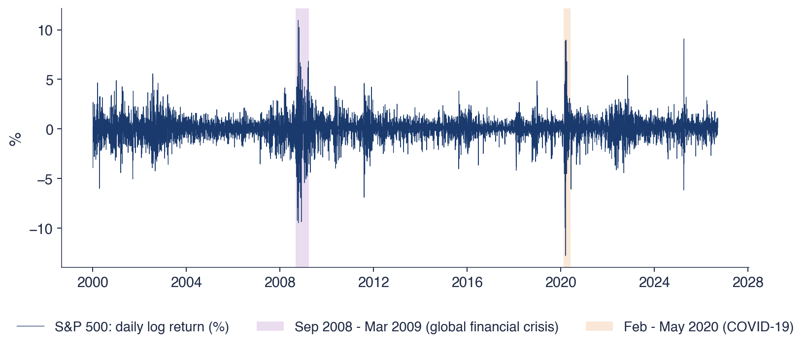
 SFM_ch9_volatility_markets