Bucharest University of Economic Studies IDA Institute Digital Assets Blockchain Research Center AI4EFin Artificial Intelligence for Energy Finance Romanian Academy, Institute for Economic Forecasting MSCA Digital Finance
A risk manager has to answer two questions every day: how much can the portfolio lose tomorrow, and was yesterday's answer right? Value at Risk (VaR) answers the first with a quantile of the loss distribution, expected shortfall (ES) with the average loss beyond that quantile, and backtesting answers the second by comparing the forecasts with the losses that actually occurred. Since 1996 these three tools have also been the language of bank regulation: the Basel rules set market-risk capital from a bank's own VaR or ES and raise it when the model fails its backtest.
The chapter builds the tools on daily data from 2000 to 2026 and judges them in two storms, the financial crisis of 2008 and the COVID-19 crash of 2020. On the S&P 500, the historical VaR 1% is 3.46% and the ES 2.5% is 3.76%, while a Normal distribution fitted to the same returns gives 2.80% and 2.81%. From September 2008 to March 2009, a rolling Normal VaR 1% of the S&P 500 was exceeded on 21 of 146 days, where a correct model would have produced about 1.5 exceptions; a VaR built on a GARCH volatility forecast was exceeded on 5 days.
The chapter therefore combines the two previous strands of the course: the tails of Chapter 5 and the volatility forecasts of Chapter 9. It shows that the choice of tail distribution matters less than tracking today's volatility, that correlation understates the risk of joint crashes, and that one year of data separates a good risk model from a bad one only roughly.
Daily log returns of the S&P 500 (%) in 2007–2009 (left) and 2019–2021 (right), with minus the VaR 1% forecasts of four methods: historical simulation (HS) and the Normal distribution on a 500-day window, GARCH-t and filtered historical simulation (FHS); dots mark the days on which the HS VaR was exceeded.
Learning outcomes
Define VaR and ES at a tail probability \(\alpha\) (VaR 1%, ES 2.5%) and compute them for the Normal and the Student-t distribution.
State the axioms of a coherent risk measure and show with a counterexample that VaR is not subadditive.
Estimate VaR and ES by historical simulation, parametric methods, Cornish–Fisher, EVT, GARCH and filtered historical simulation.
Compute the VaR of a portfolio and explain why correlation does not measure the risk of joint crashes.
Backtest a VaR model with the Kupiec and Christoffersen tests and with the Basel traffic light.
Chapter plan
Measuring Tail RiskThe 4:15 report, RiskMetrics, the Basel rules and the two crises used as stress tests.
VaR and ES: DefinitionsLosses, horizon and level; VaR as a quantile, ES as a tail average; closed forms for the Normal and the Student-t; the square-root-of-time rule.
Coherent Risk MeasuresThe four axioms, a counterexample in which VaR penalises diversification, and elicitability.
Estimating VaR and ESHistorical simulation and its precision, the Normal, Student-t, Cornish–Fisher and EVT methods on six series.
BacktestingThe hit sequence, the Kupiec and Christoffersen tests, the Basel traffic light and the backtest of ES.
AI for Scientific DiscoveryAn open question on tail dependence between Bucharest and world markets, the role of AI and the checks.
SummaryKey results, formulas and self-check questions.
Measuring Tail Risk
The section tells how a single daily number came to summarise the risk of a bank. It starts with the request of J.P. Morgan's chairman for a daily report, follows VaR from the RiskMetrics document of 1994 to the Basel capital rules of 1996 and 2019, and introduces the two crises, 2008 and 2020, in which every method of the chapter is tested.
Around 1990, Dennis Weatherstone, the chairman of J.P. Morgan, asked for a single number, delivered every day at 4:15 pm after the close of trading, that would say how much the bank could lose over the next day. The bank's trading desks held positions in bonds, currencies, equities and derivatives, and no individual report could add them up. The answer became the Value at Risk (VaR): a loss that is exceeded only with a small probability over a given horizon.
In October 1994 the bank published its methodology and the data needed to apply it free of charge, under the name RiskMetrics; the fourth edition of the technical document is J.P. Morgan/Reuters (1996). The method was deliberately simple: Normal returns, a volatility estimated by an exponentially weighted moving average (EWMA, the estimator of Chapter 8) and a VaR at a tail probability of 5% over one day.
The publication turned VaR into a common language. Banks, regulators and fund managers could now state their market risk in the same units, a loss in currency at a given probability, and compare positions that had nothing else in common. The simplicity that made the method popular also contains its two weak points, which the chapter examines in turn: the Normal distribution has too thin a tail, and a quantile says nothing about the size of the losses beyond it.
In brief
Around 1990: J.P. Morgan's chairman, Dennis Weatherstone, asks for one number, every day at 4:15 pm, summarising how much the bank could lose the next day
the answer became the value at risk (VaR): a loss that is exceeded only with a small probability
October 1994: the methods and data are published free of charge as RiskMetrics J.P. Morgan/Reuters (1996)
Normal returns, EWMA volatility (Chapter 8), VaR at a 5% tail probability over one day
VaR became the common language of banks, regulators and fund managers
The Basel Committee on Banking Supervision (BCBS), hosted by the Bank for International Settlements (BIS) in Basel, sets the international standards for bank capital (history of the Basel Committee). In 1996 it allowed banks to compute the capital for market risk with their own internal VaR models (BCBS, 1996a). The rule uses VaR 1% over 10 days, multiplied by a factor of at least 3, and the factor increases when the model fails its backtest, that is, when actual losses exceed the VaR too often (BCBS, 1996b).
In 2019 the Fundamental Review of the Trading Book (FRTB) replaced VaR 1% with ES 2.5% as the basis of the capital charge (BCBS, 2019); the current rule is chapter MAR33 of the Basel Framework (BCBS, 2023b). The change answers the main criticism of VaR: a quantile ignores how bad the losses beyond it are, while ES averages them.
Backtesting did not move to ES. Under chapter MAR32 of the Basel Framework (BCBS, 2023a), banks still count the days on which the loss exceeded the VaR forecast, at the level of the bank and of each trading desk. The reason is statistical and appears in the Coherent Risk Measures section: a VaR forecast can be checked against realised losses on its own, while an ES forecast can only be checked together with a VaR forecast.
In brief
The BCBS (Basel Committee on Banking Supervision) sits at the BIS (Bank for International Settlements) in Basel history of the Basel Committee
1996: banks may compute market-risk capital with their own VaR models BCBS (1996a)
rule: VaR 1% over 10 days, times a multiplier of at least 3; the multiplier grows when the model fails the backtest BCBS (1996b)
2019: the FRTB (Fundamental Review of the Trading Book) BCBS (2019)
capital from ES 2.5% instead of VaR 1% (MAR33, BCBS (2023b)); backtesting still counts VaR exceptions (MAR32, BCBS (2023a))
The photographs show the two crises that frame the chapter: the headquarters of Lehman Brothers in New York on 15 September 2008, the day of its bankruptcy, and the deserted financial district of New York on 25 March 2020, during the COVID-19 lockdown. The worst day of the S&P 500 since 2000 came in the second crisis: a daily log return of −12.8% on 16 March 2020.
A Normal model with the sample volatility gives such a day a probability that is practically zero; Chapter 5 measured how far from zero. A risk measure built on that model would have been useless exactly when it was needed.
The chapter therefore uses September 2008 – March 2009 and February – May 2020 as stress tests for every method. A method that gives sensible numbers in calm years but fails in these two periods does not measure tail risk; it measures ordinary variation.
The worst day of the S&P 500 since 2000: \(-12.8\%\) on 16 March 2020; a Normal model with the sample volatility gives such a day a probability of practically zero
A risk measure must be judged in such periods: we use 2008 and 2020 as stress tests throughout the chapter
Section summary
VaR was born as a practical answer to a management question and became a regulatory standard within a few years: Basel 1996 based market-risk capital on VaR 1% over 10 days, and the FRTB of 2019 replaced it with ES 2.5% while keeping the count of VaR exceptions as the backtest. The next section defines both measures precisely and computes them for the S&P 500.
VaR and ES: Definitions
The section defines VaR and ES as functions of the distribution of the profit and loss, computes them first on a toy sample of 100 days and then on 26 years of S&P 500 returns, derives the closed forms for the Normal and the Student-t distributions, and examines the rule that scales a one-day VaR to ten days.
A risk measure needs three ingredients. The first is the random variable \(X\): the profit and loss (P&L) or the return of a position over a horizon \(h\); in this chapter \(h\) is one day and \(X\) is the daily log return in percent. The loss is \(L = -X\), a positive number when the position loses money. Both conventions appear in the literature, and most errors in practice come from mixing them.
The second ingredient is the level \(\alpha\), the tail probability, for example \(\alpha = 1\%\) or \(\alpha = 2.5\%\). The course writes VaR 1% and ES 2.5%: the number in the name is always the probability of the tail. Regulatory texts and software often speak of "VaR 99%", naming the complementary confidence level; the two names describe the same number, but the course uses only the tail probability, so that a smaller number always means a more extreme loss.
The third ingredient is the quantile. The quantile of order \(\alpha\) of \(X\) is \(q_\alpha(X) = \inf\{x : P(X \le x) > \alpha\}\), the definition of Chapter 2 that also works for discrete distributions. For a continuous distribution function \(F\) it is simply \(q_\alpha = F^{-1}(\alpha)\). For small \(\alpha\) the quantile of returns is a negative number: the return below which the worst \(\alpha\) of the days fall.
In brief
\(X\): the P&L (profit and loss) or the return of a position over a horizon \(h\) (here one day, in %)
the loss is \(L = -X\): a positive number when the position loses money
The level\(\alpha\) is the probability of the tail: \(\alpha = 1\%\) or \(\alpha = 2.5\%\)
we write VaR 1% and ES 2.5%: the number in the name is always the tail probability
\(q_\alpha(X) = \inf\{x : P(X \le x) > \alpha\}\): the \(\alpha\)-quantile of \(X\) (Chapter 2)
for a continuous distribution function \(F\): \(q_\alpha = F^{-1}(\alpha)\), a negative number for small \(\alpha\)
The Value at Risk at level \(\alpha\) is the negative of the \(\alpha\)-quantile of the P&L:
\[\mathrm{VaR}_\alpha(X) = -q_\alpha(X).\]
(10.1)
The minus sign turns the quantile into a positive loss. The definition implies \(P(L > \mathrm{VaR}_\alpha) \le \alpha\): the loss exceeds the VaR with probability at most \(\alpha\). A daily VaR 1% of 3% therefore says that a loss larger than 3% occurs on about one day in a hundred. In money, a position worth \(W\) has a VaR of \(W \times \mathrm{VaR}(\%)/100\).
What VaR does not say matters as much. It says nothing about the size of the losses beyond it: two positions with the same 1% quantile, one of which loses 4% on its bad days and the other 40%, have the same VaR. And VaR is not the maximum loss. By construction it is exceeded on about a fraction \(\alpha\) of the days; a VaR that is never exceeded is not a prudent VaR but a wrong one, as the backtests of the Backtesting section show.
Expected shortfall answers the question VaR leaves open: how large is the loss on the bad days? It is defined as the average of the VaR over all levels below \(\alpha\):
where the integration variable \(u\) runs over the tail levels from 0 to \(\alpha\). For a continuous distribution the definition reduces to \(\mathrm{ES}_\alpha = -E[X \mid X \le q_\alpha(X)]\): the average loss on the worst \(\alpha\) of the days. The same quantity appears under other names, conditional VaR (CVaR), tail VaR (TVaR) or expected tail loss; for continuous distributions they coincide.
Two properties follow from the definition. Because the quantiles \(q_u\) for \(u < \alpha\) all lie below \(q_\alpha\), their average does too, so \(\mathrm{ES}_\alpha \ge \mathrm{VaR}_\alpha\) at the same level. And ES looks inside the tail: two distributions with the same VaR but different tails, one ending abruptly and one with rare catastrophic losses, have different ES. The integral form (10.2) is the general definition; it remains valid for discrete distributions, where the conditional expectation can give a different and less well-behaved number.
In brief
Definition: \(\mathrm{ES}_\alpha(X) = -\dfrac{1}{\alpha}\displaystyle\int_0^\alpha q_u(X)\,du\): the average of the VaRs at all levels below \(\alpha\)
for a continuous distribution: \(\mathrm{ES}_\alpha = -E[X \mid X \le q_\alpha(X)]\), the average loss on the worst \(\alpha\) of the days
\(u\): the integration variable, a tail level running from 0 to \(\alpha\)
other names: CVaR (conditional VaR), TVaR (tail VaR), expected tail loss
Properties
\(\mathrm{ES}_\alpha \ge \mathrm{VaR}_\alpha\) at the same level \(\alpha\)
ES looks inside the tail: two distributions with the same VaR but different tails have different ES
With a sample, the quantile is replaced by an order statistic. A position has 100 daily returns, and the five worst are −6.1%, −4.8%, −4.2%, −3.9% and −3.5%. The empirical quantile of level \(\alpha\) is the \(k\)-th smallest return, with \(k = \lceil n\alpha \rceil\), where \(\lceil\cdot\rceil\) rounds up to the next integer.
For VaR 1%, \(k = \lceil 100 \times 0.01 \rceil = 1\): the empirical quantile is the worst return, and \(\mathrm{VaR}_{1\%} = 6.1\%\). A single observation decides this estimate, so with 100 days it is very imprecise: a different sample of 100 days would almost surely have a different worst day. For ES 2.5%, \(k = \lceil 2.5 \rceil = 3\), and the estimate is the average of the three largest losses, \(\mathrm{ES}_{2.5\%} = (6.1 + 4.8 + 4.2)/3 = 5.03\%\), while \(\mathrm{VaR}_{2.5\%}\) is the third largest loss, 4.2%.
Translated into money, a position of 1 million lei has a VaR 1% of 61,000 lei: on one day in a hundred, the loss is larger. The example also shows why ES at 2.5% and VaR at 1% are natural partners: ES 2.5% uses three observations where VaR 1% uses one, and its value, 5.03%, lies between the worst and the third-worst loss.
In brief
A position has 100 daily returns; the five worst are \(-6.1\), \(-4.8\), \(-4.2\), \(-3.9\), \(-3.5\) (in %)
empirical quantile at level \(\alpha\): the \(k\)-th smallest return, \(k = \lceil n\alpha \rceil\) (\(\lceil\cdot\rceil\): rounding up)
VaR 1%: \(k = \lceil 100 \times 0.01 \rceil = 1\), so \(\mathrm{VaR}_{1\%} = 6.1\%\)
one observation decides VaR 1%: with 100 days the estimate is very imprecise
ES 2.5%: \(k = \lceil 2.5 \rceil = 3\); the average of the three worst losses
Question for the room What happens to the Normal VaR 1% relative to the historical one when we move to the other five series?
Answer
It stays below the historical one everywhere, by 14–24%: 22% for the DAX, 23% for the BET, 24% for Bitcoin, 22% for TLV, 14% for SNP (S&P 500: 19%). Two parameters, the mean and the standard deviation, cannot describe a heavy tail: the Normal distribution puts too little probability beyond 2.3 standard deviations.
Question for the room The VaR 1% of the 10-day S&P 500 returns: is it above or below √10 × the one-day VaR (10.93%)?
Answer
Below: 10.37%, that is 3.00 times the one-day VaR, against √10 = 3.16. The sum of 10 heavy-tailed returns is closer to the Normal distribution (CLT), and the first-order autocorrelation of the S&P 500 returns is −0.10, so consecutive days partly offset each other. For the BET the ratio is 3.86, above √10: its autocorrelation is +0.11.
Question for the room With the last 250 days of the S&P 500, which worst day does the historical VaR 1% rest on?
Answer
The third: k = ⌈250 × 0.01⌉ = ⌈2.5⌉ = 3. With 250 days, VaR 1% depends on 3 observations and ES 2.5% on 7 (⌈6.25⌉); on the whole sample of 6,714 days, VaR 1% is the 68th worst day.
Question for the room On the last 500 days of the S&P 500, how many times wider is the 95% bootstrap interval for VaR 1% than on all 6,714 days?
Answer
About 6 times: [1.99, 4.96], that is 2.97 percentage points, against [3.18, 3.66], that is 0.48. The √n rule would give √(6,714/500) = 3.7; the interval is wider because VaR 1% rests on the 5th worst day, and the five worst days of the window are far apart. On the last 250 days the interval is only 1.12 points wide: a window without extreme days looks precise although it has fewer observations.
Question for the room S&P 500: S = −0.35, K = 10.7. How does the Cornish–Fisher VaR 1% compare with the historical one (3.46%)?
Answer
It is almost double: 6.08%. The kurtosis term (z³ − 3z)K/24 = −2.49 alone adds more than the distance between the Normal and the empirical quantile; the expansion is a small correction around the Normal distribution and no longer holds when K exceeds 10.
Question for the room We raise the EVT threshold of the S&P 500 from the 90% to the 97.5% quantile of the losses. What does the EVT VaR 1% do?
Answer
It changes little: 3.56% at 90%, 3.54% at 95%, 3.50% at 97.5% (3.59% at 85%). ξ̂ rises from 0.16 to 0.23, but at 1% we are still close to the data used; the difference shows at 0.1%, where the EVT VaR moves from 6.91% to 7.13%.
Question for the room On the S&P 500 since 2000, the historical VaR 1% is 3.46%. What is the historical ES 2.5%?
Answer
3.76%: the average of the worst 168 days, with the sign changed. VaR 2.5% = 2.51% is only the edge of this tail, while ES 2.5% averages the whole tail, including the days of 2008 and 2020. ES 2.5% and VaR 1% are close (3.76% against 3.46%), which is why FRTB could replace VaR 1% by ES 2.5% without changing the capital level much (BCBS (2019); BCBS (2023b)).
The histogram shows the 6,714 daily log returns of the S&P 500 since 2000. The shaded area is the worst 2.5% of the days. The solid line marks minus the historical VaR 1%, at −3.46%, and the dashed line minus the ES 2.5%, at −3.76%; the historical VaR 2.5%, the right edge of the shaded area, is 2.51%.
The two lines answer different questions. VaR 1% is a single point of the tail: 1% of the days lie to its left, wherever they lie. ES 2.5% averages the whole shaded tail, including the extreme days of 2008 and 2020 that are barely visible as isolated bars far to the left; if those days had been twice as bad, the VaR 1% would be unchanged while the ES would rise.
For a position of 1 million lei in the index, the two numbers translate into a VaR 1% of about 34,552 lei and an ES 2.5% of about 37,613 lei. The ES 2.5% is larger than the VaR 1% even though it refers to a less extreme probability, because it averages the losses beyond the 2.5% quantile, and some of these losses are much larger than 3.46%.
In brief
Daily log returns since 2000 (6 714 days); historical estimates: VaR 1% \(= 3.46\%\), VaR 2.5% \(= 2.51\%\), ES 2.5% \(= 3.76\%\)
Interpretation: ES 2.5% averages the whole shaded tail, including the extreme days of 2008 and 2020; VaR 1% is one point in that tail
For a position of 1 million RON in the index: VaR 1% about 34 552 RON, ES 2.5% about 37 613 RON
If \(X \sim N(\mu, \sigma^2)\), both measures have closed forms. With \(z_\alpha = \Phi^{-1}(\alpha)\) the standard Normal quantile, where \(\Phi\) and \(\varphi\) are the distribution function and the density of \(N(0, 1)\),
The ES formula rests on the tail mean of the standard Normal, \(E[Z \mid Z \le z] = -\varphi(z)/\Phi(z)\). The derivation uses \(\varphi'(z) = -z\varphi(z)\): integrating \(t\varphi(t)\) from \(-\infty\) to \(z\) gives \(-\varphi(z)\), and dividing by \(P(Z \le z) = \Phi(z) = \alpha\) gives the conditional mean.
The constants are worth knowing: \(z_{0.01} = -2.326\),\(z_{0.025} = -1.960\),\(\varphi(z_{0.025}) = 0.0584\), and the ES factor at 2.5% is \(\varphi(z_{0.025})/0.025 = 2.338\). With \(\mu = 0\), the ratio of ES 2.5% to VaR 1% is \(2.338/2.326 = 1.005\): for Normal returns the two measures are practically equal. This is why the FRTB chose ES 2.5% to replace VaR 1%: for Normal data the capital charge stays about the same, and for heavy-tailed data, where the ES 2.5% exceeds the VaR 1%, it rises.
In brief
\(X \sim N(\mu, \sigma^2)\), \(z_\alpha = \Phi^{-1}(\alpha)\) (\(\Phi\), \(\varphi\): distribution function and density of \(N(0,1)\))
The sample moments of the daily S&P 500 returns since 2000 are \(\hat\mu = 0.025\%\) and \(\hat\sigma = 1.21\%\). Inserted into (10.3), they give the Normal VaR 1% \(= -(0.025 - 2.326 \times 1.21) = -0.025 + 2.822 = 2.80\%\) and the Normal ES 2.5% \(= -0.025 + 2.338 \times 1.21 = -0.025 + 2.836 = 2.81\%\).
The data tell a different story. Historical simulation gives VaR 1% = 3.46% and ES 2.5% = 3.76%. The Normal VaR 1% is 19% too small, because the Normal tail is too thin (Chapter 2). The Normal ES 2.5% is even further from the data, about a quarter below the historical value, because the Normal tail has nothing like the extreme days that the historical average includes.
Two parameters, a mean and a standard deviation, are fitted to the centre of the distribution, where most of the observations are; they cannot also describe the tail. The methods of the following sections take one of two routes: they change the distribution (Student-t, Cornish–Fisher, EVT) or they change the data used (historical simulation, volatility filtering).
In brief
Sample moments of the daily returns since 2000: \(\hat\mu = 0.025\), \(\hat\sigma = 1.21\) (in %)
The Student-t distribution of Chapter 2 has a power-law tail. Write \(X = m + s\,T\) with \(T \sim t_\nu\), a location \(m\), a scale \(s\) and \(\nu\) degrees of freedom; let \(t_\alpha = t_\nu^{-1}(\alpha)\) be the quantile and \(f_\nu\) the density of \(t_\nu\). Then
The condition \(\nu > 1\) is needed for the mean, and hence the ES, to exist. The scale \(s\) is not the standard deviation: the variance of \(X\) is \(s^2\nu/(\nu - 2)\), so a standardised t with variance 1 has \(s = \sqrt{(\nu - 2)/\nu}\). This standardisation reappears in the GARCH-t model of the conditional VaR section.
Fitted to the S&P 500 by maximum likelihood, the distribution has location \(\hat m = 0.068\), scale \(\hat s = 0.703\) and \(\hat\nu = 2.67\) degrees of freedom. The quantile is \(t_{0.01} = -5.023\), so the VaR 1% \(= -(0.068 + 0.703 \times (-5.023)) = 3.46\%\), exactly the historical value. The ES factor is 5.720, so the ES 2.5% \(= -0.068 + 0.703 \times 5.720 = 3.95\%\), above the historical 3.76%. With \(\nu < 3\) the fitted tail is very heavy: it matches the 1% quantile, but beyond it the t distribution places more mass than the data show.
In brief
\(X = m + s\,T\), \(T \sim t_\nu\) (location \(m\), scale \(s\), \(\nu\) degrees of freedom, Chapter 2); \(t_\alpha = t_\nu^{-1}(\alpha)\), \(f_\nu\) the density of \(t_\nu\)
Regulatory VaR has a 10-day horizon, while data and models are daily. The square-root-of-time rule bridges the gap: \(\mathrm{VaR}^{(h)} \approx \sqrt{h}\,\mathrm{VaR}^{(1)}\). The rule is exact for i.i.d. Normal returns with mean zero, because the \(h\)-day return is then Normal with standard deviation \(\sigma\sqrt{h}\) and every quantile scales by \(\sqrt{h}\). Basel 1996 asked for a 10-day VaR, usually obtained from the one-day VaR by the factor \(\sqrt{10} = 3.162\).
For the S&P 500, the historical one-day VaR 1% is 3.46%, and the rule gives \(3.162 \times 3.46 = 10.93\%\) over 10 days. The historical VaR 1% of overlapping 10-day returns is 10.37%, somewhat smaller: the ratio is 3.00, below \(\sqrt{10}\). The difference is not an accident of the sample but the result of three features of real returns.
The first is heavy tails. The sum of 10 heavy-tailed returns is closer to Normal than each of them (the central limit theorem, CLT), so its kurtosis is lower and the ratio of its 1% quantile to the daily one is below \(\sqrt{10}\). The second is volatility clustering (Chapter 9): after a quiet day volatility tends to rise back to its long-run level, so the 10-day risk is more than \(\sqrt{10}\) times today's risk; after a turbulent period it tends to fall, and the 10-day risk is less. The third is autocorrelation. The variance of a 10-day sum is \(\sigma^2\bigl(10 + 2\sum_{k=1}^{9}(10-k)\rho_k\bigr)\), so a negative first-order autocorrelation lowers it and a positive one raises it. The S&P 500 has \(\hat\rho_1 = -0.10\): consecutive days partly offset each other, which adds to the effect of the heavy tails. The BET has \(\hat\rho_1 = +0.11\) (the non-synchronous trading of its constituents), and its ratio is 3.86, above \(\sqrt{10}\). The rule is a convention of regulation, not a property of the data.
volatility clustering: after a calm day the 10-day risk is larger than \(\sqrt{10}\) times today's, after a storm smaller (Chapter 9)
Section summary
VaR (10.1) is a quantile of the loss and ES (10.2) the average loss beyond it. On the S&P 500 since 2000 the historical values are VaR 1% = 3.46% and ES 2.5% = 3.76%; the Normal distribution gives 2.80% and 2.81%, while a Student-t matches the VaR and overshoots the ES. The next section asks which properties a good risk measure should have and finds that VaR lacks one of them.
Coherent Risk Measures
The section judges VaR and ES by two theoretical criteria. The first, coherence, asks whether a risk measure behaves sensibly when positions are scaled or combined; the four axioms of Artzner, Delbaen, Eber and Heath define it, and a counterexample with two bonds shows that VaR can violate it. The second, elicitability, asks whether forecasts of the measure can be compared with outcomes, and here the ranking of the two measures reverses.
Artzner et al. (1999) define a risk measure \(\rho\) as a map from a loss \(L\) to the amount of capital that makes the position acceptable to a regulator. They call \(\rho\)coherent if it satisfies four axioms. Monotonicity: if \(L_1 \le L_2\) in every state of the world, then \(\rho(L_1) \le \rho(L_2)\). Translation invariance: \(\rho(L + c) = \rho(L) + c\) for a certain amount \(c\), so adding a sure loss raises the capital by exactly that amount. Positive homogeneity: \(\rho(\lambda L) = \lambda\rho(L)\) for \(\lambda > 0\), so doubling a position doubles its capital. Subadditivity: \(\rho(L_1 + L_2) \le \rho(L_1) + \rho(L_2)\).
The first three axioms are almost uncontroversial. Subadditivity carries the economic content: merging two positions never creates risk, so diversification never adds risk. It has a practical consequence for a bank: the sum of the capital computed separately for each division is an upper bound for the capital of the whole bank, and the capital can be allocated division by division. A measure that is not subadditive could make a merged bank look riskier than its two halves, and it would reward splitting a portfolio artificially to lower the capital.
The photograph shows Freddy Delbaen, one of the four authors, in 1997. The axioms were published in 1999 in Mathematical Finance and changed the question about risk measures from "which number is intuitive?" to "which properties must the number have?".
In brief
Artzner et al. (1999): a risk measure \(\rho\) maps a loss \(L\) to the capital that makes it acceptable; \(\rho\) is coherent if
Two independent bonds each lose 100 if the issuer defaults, which happens with probability 4%, and 0 otherwise; the level is \(\alpha = 5\%\). For one bond, \(P(L > 0) = 4\% \le 5\%\), so the 5% quantile of the loss is 0 and \(\mathrm{VaR}_{5\%} = 0\) for each bond. A risk manager using VaR would see no risk in either bond.
For the portfolio of both bonds, the loss is 200 if both default, with probability \(0.04^2 = 0.16\%\), and 100 if exactly one defaults, with probability \(2 \times 0.04 \times 0.96 = 7.68\%\). Now \(P(L > 0) = 7.84\% > 5\%\), so the VaR of the portfolio is 100. Since \(\mathrm{VaR}_{5\%}(L_1 + L_2) = 100 > 0 + 0\), VaR penalises diversification: holding both bonds appears riskier than the sum of holding each.
ES 5% is the average of the worst 5% of the outcomes. For one bond, the worst 5% consist of the 4% of default states with loss 100 and 1% of the states with loss 0, so \(\mathrm{ES}_{5\%} = (4\% \times 100 + 1\% \times 0)/5\% = 80\). For the portfolio, the worst 5% consist of the 0.16% with loss 200 and 4.84% with loss 100, so \(\mathrm{ES}_{5\%} = (0.16\% \times 200 + 4.84\% \times 100)/5\% = 103.2\). Since \(103.2 \le 80 + 80\), ES is subadditive here, and it sees the default risk of each bond, which VaR ignores entirely.
In brief
Two independent bonds; each loses 100 with probability 4% (default) and 0 otherwise; level \(\alpha = 5\%\)
one bond: \(P(L > 0) = 4\% \le 5\%\), so \(\mathrm{VaR}_{5\%} = 0\) for each
Both bonds: \(P(L = 200) = 0.16\%\), \(P(L = 100) = 7.68\%\), so \(P(L > 0) = 7.84\% > 5\%\)
ES satisfies all four axioms (Acerbi & Tasche, 2002). The reason is visible in (10.2): ES is an average of quantiles over the tail, and averages respect sums. More precisely, ES can be written as the largest expected loss over a set of reweighted scenarios, and the maximum of a sum is never larger than the sum of the maxima.
VaR satisfies the first three axioms; subadditivity can fail. It fails for discrete losses, such as credit losses and the bonds of the previous example, and for extremely heavy tails, with a tail index below 1 (Chapter 5), where the mean loss is infinite. It holds for elliptical distributions such as the Normal and the Student-t, and Daníelsson et al. (2013) show that in practice it holds for most equity returns, whose tail index lies well above 1.
ES pays for coherence with a stronger requirement: it needs a finite mean loss, while VaR exists for every distribution. For daily equity returns, whose tail index is around 3, this is not a constraint; for some operational or insurance losses it can be.
A statistic is elicitable if some loss function, or scoring function, is minimised in expectation by its true value (Gneiting, 2011). The mean is elicitable through the squared error, the median through the absolute error. Elicitability matters because it allows competing forecasts to be ranked: the forecaster with the smaller average score is the better one, and no forecaster can lower the expected score by reporting anything other than the true value.
VaR is elicitable. The scoring function is the quantile, or pinball, loss
where \(v\) is the VaR forecast, \(x\) the realised return and \(\mathbf{1}\{\cdot\}\) equals 1 if the event occurs and 0 otherwise. Its expectation is minimised where \(P(X < -v) = \alpha\), that is at \(v = \mathrm{VaR}_\alpha\). Two VaR models can therefore be compared by the average quantile loss of their forecasts, as the Backtesting section does.
ES alone is not elicitable (Gneiting, 2011): no scoring function is minimised in expectation by the true ES. The pair (VaR, ES), however, is jointly elicitable (Fissler & Ziegel, 2016). The consequence is practical: forecasts of ES are tested together with forecasts of VaR, as in the ES backtest at the end of the Backtesting section. Coherence favours ES, elicitability favours VaR, and the Basel rules use both: ES for capital, VaR exceptions for the backtest.
In brief
A statistic is elicitable if some loss (scoring) function is minimised, on average, by its true value Gneiting (2011)
the mean: squared error; the median: absolute error
VaR is elicitable: the quantile (pinball) loss \(S(v, x) = (\alpha - \mathbf{1}\{x < -v\})(x + v)\)
\(v\): the VaR forecast; \(x\): the realised return; \(\mathbf{1}\{\cdot\}\): 1 if the event occurs, 0 otherwise
two VaR models can be compared by their average quantile loss
consequence: ES forecasts are tested together with VaR forecasts (Section 7)
Section summary
ES is coherent; VaR is not always subadditive and can penalise diversification, as the two-bond example shows with a portfolio VaR of 100 against individual VaRs of 0. VaR is elicitable through the pinball loss (10.5), while ES is elicitable only together with VaR. The next section turns from properties to estimation.
Estimating VaR and ES
The section compares five unconditional methods: historical simulation, the Normal and Student-t distributions, the Cornish–Fisher expansion and EVT. It computes each step by step for the S&P 500, measures the sampling error of a historical VaR with the bootstrap, and compares all methods on six series: the S&P 500, the DAX and the BET from 2000, Bitcoin from 2014, and two stocks of the Bucharest Stock Exchange (BVB), Banca Transilvania (TLV) and OMV Petrom (SNP), from 2010.
The table lists the five methods with their assumption and their weak point. Historical simulation (HS) assumes that the past window is a sample from tomorrow's distribution; it has few points in the tail and cannot produce a loss beyond the worst day in the window. The Normal method assumes Normal returns and has tails that are far too thin. The Student-t method allows heavy tails but forces one shape on both tails. The Cornish–Fisher method corrects the Normal quantile for skewness and kurtosis and breaks down when the kurtosis is large. EVT fits a generalised Pareto distribution (GPD) above a high threshold, as in Chapter 5, and its weak point is the choice of the threshold.
"Unconditional" means that the method gives the same VaR on every day of the estimation window: it describes the distribution of returns averaged over calm and turbulent periods. The conditional methods of the next section instead scale the forecast with today's volatility.
All methods use daily log returns in percent (Chapter 1) and report VaR and ES as positive losses. This common convention makes the numbers directly comparable across methods and series.
In brief
Method
Assumption
Weak point
historical simulation (HS)
the past window is a sample of tomorrow
few tail points; nothing beyond the worst day
Normal
returns are Normal
tails far too thin
Student-t
returns are Student-t
one tail shape for both tails
Cornish–Fisher
Normal quantile corrected by skewness and kurtosis
Historical simulation is the simplest estimator. Take the last \(n\) returns \(r_{t-n+1}, \dots, r_t\) and sort them, \(r_{(1)} \le \dots \le r_{(n)}\). Then
No distribution is assumed: the empirical distribution of the window is the forecast. For the S&P 500 since 2000, \(n = 6{,}714\). The VaR 1% uses \(k = \lceil 67.14 \rceil = 68\), and the 68th worst day is a loss of 3.46%. The ES 2.5% is the average of the worst \(\lceil 167.85 \rceil = 168\) days, 3.76%.
The window length \(n\) is a trade-off. A short window of 250 days reacts to recent events, but its VaR 1% is the third worst return, \(k = \lceil 2.5 \rceil = 3\), and rests on three observations. A long window, here all the data, gives a stable estimate that does not react to today's volatility at all.
A specific artefact of a fixed window is the ghost effect. A crash day changes the VaR when it enters the window, which is reasonable, and changes it again, abruptly, \(n\) days later when it leaves the window, although nothing happened on that day. With a 500-day window, a crash stays in the estimate for about two years, as the rolling forecasts of the conditional VaR section show.
In brief
Algorithm: take the last \(n\) returns \(r_{t-n+1}, \dots, r_t\), sort them: \(r_{(1)} \le \dots \le r_{(n)}\)
A VaR estimate is a statistic and has a sampling error. The bootstrap of Chapter 2 measures it: resample the \(n\) returns with replacement 2000 times, recompute VaR and ES on each resample, and read the 2.5% and 97.5% quantiles of the 2000 values as a 95% interval.
With all 6,714 S&P 500 days, the VaR 1% of 3.46% has the 95% interval [3.18%, 3.66%], and the ES 2.5% of 3.76% has [3.46%, 4.07%]. With the last 500 days only, the VaR 1% is 2.75% with the interval [1.99%, 4.96%], and the ES 2.5% is 2.94% with [2.14%, 3.82%]. With two years of data, the interval for the VaR 1% is almost three percentage points wide, because the estimate rests on the five worst days, \(k = \lceil 500 \times 0.01 \rceil = 5\). The interval of the ES is narrower, since an average of 13 observations varies less than a single order statistic.
The intervals set a scale for every comparison that follows. A difference between two methods that is smaller than the bootstrap interval does not show that one method is better; it may be sampling noise. The resampling treats the days as independent, so with volatility clustering the true uncertainty is, if anything, larger.
In brief
A VaR estimate is a statistic: it has a sampling error; we measure it with the bootstrap (Chapter 2)
resample the \(n\) returns with replacement 2000 times, recompute VaR and ES, read the 2.5% and 97.5% quantiles
S&P 500, all 6 714 days: VaR 1% \(= 3.46\%\), 95% interval [3.18, 3.66]; ES 2.5% \(= 3.76\%\), [3.46, 4.07]
last 500 days: VaR 1% \(= 2.75\%\), [1.99, 4.96]; ES 2.5% \(= 2.94\%\), [2.14, 3.82]
With two years of data the interval of VaR 1% is wider than 2 percentage points: VaR 1% rests on 5 observations
Interpretation: differences between methods smaller than the bootstrap interval are not evidence that one method is better
Cornish & Fisher (1938) correct the Normal quantile \(z = z_\alpha\) with the skewness \(S\) and the excess kurtosis \(K\), the kurtosis coefficient minus 3:
The expansion is a series in the higher cumulants around the Normal quantile. At \(z_{0.01} = -2.326\), a negative skewness \(S\) and a positive excess kurtosis \(K\) both push the quantile further into the left tail, so the VaR rises above the Normal value.
For the S&P 500, \(S = -0.35\) and \(K = 10.7\). The kurtosis term alone is \((z^3 - 3z)K/24 \approx -2.50\), larger than the Normal quantile itself, and the corrected quantile is \(z_{CF} = -5.03\), which gives a VaR 1% of 6.08%, against the historical 3.46%. The correction has overshot by more than the Normal method undershot.
The expansion is a small-correction device: it is accurate when the distribution is close to Normal and the correction terms are small compared with \(z\). With an excess kurtosis above 10, the terms are no longer small and the expansion lies far above the correct value. The method is useful only when \(|S|\) and \(K\) are moderate, for example for monthly returns or for diversified portfolios.
In brief
Cornish & Fisher (1938): correct the Normal quantile \(z = z_\alpha\) with the skewness \(S\) and the excess kurtosis \(K\) (kurtosis minus 3)
The peaks-over-threshold (POT) method of Chapter 5 models only the tail. With the losses \(L = -r\) and a threshold \(u\) set at the 90% quantile of the losses, as in McNeil & Frey (2000), the excesses \(L - u\) above \(u\) follow approximately a GPD with shape \(\xi\) and scale \(\beta\). The tail estimator then gives
where \(n\) is the number of days and \(N_u\) the number of excesses. The ratio \(n\alpha/N_u\) compares the target tail probability with the share of days above the threshold; a shape \(\xi > 0\) means a heavy, Pareto-type tail.
For the S&P 500, \(u = 1.26\%\),\(N_u = 672\) excesses (10.0% of the days), \(\hat\xi = 0.164\) and \(\hat\beta = 0.820\). For VaR 1%, \(n\alpha/N_u = 0.0999\) and \(0.0999^{-\hat\xi} = 1.461\); with \(\hat\beta/\hat\xi = 4.988\), the VaR 1% is \(1.26 + 4.988 \times (1.461 - 1) = 3.56\%\). The ES 2.5% is 3.77%. Both are close to the historical values, 3.46% and 3.76%.
At 1% and 2.5% the EVT and historical estimates agree because both are driven by the same few hundred tail observations. EVT adds value further out: it smooths the tail with a two-parameter model and extrapolates beyond the worst observed day, which makes it the method for VaR 0.1% and for stress tests.
In brief
Losses \(L = -r\); threshold \(u\) = the 90% quantile of the losses McNeil & Frey (2000); excesses \(L - u\) above \(u\) follow a GPD (generalised Pareto distribution) with shape \(\xi\) and scale \(\beta\)
\(\mathrm{VaR}_\alpha = u + \dfrac{\beta}{\xi}\Big[\Big(\dfrac{n\alpha}{N_u}\Big)^{-\xi} - 1\Big]\), \(\mathrm{ES}_\alpha = \dfrac{\mathrm{VaR}_\alpha + \beta - \xi u}{1 - \xi}\) (\(N_u\): number of excesses)
\(n\): the number of days; \(n\alpha/N_u\): the tail probability relative to the share of excesses; \(\xi > 0\): a heavy tail
S&P 500: \(u = 1.26\%\), \(N_u = 672\) (10.0% of the days), \(\hat\xi = 0.164\), \(\hat\beta = 0.820\)
VaR by method, full samples, in % (K: excess kurtosis)
Question for the room At VaR 5%, is the Normal VaR still below the historical one?
Answer
No: at 5% the Normal VaR is above the historical one for all six series, by 3–16% (S&P 500: 1.97% against 1.85%). A heavy-tailed distribution with the same variance has more probability in the centre and in the far tail and less on the "shoulders": its 5% quantile is closer to 0 than the Normal one.
ES by method, full samples, in %
Question for the room For the Normal distribution, ES 2.5% / VaR 1% = 1.005. In the data, by how much does the historical ES 2.5% exceed the historical VaR 1%?
Answer
By 1.5–10.5%, depending on the series (DAX 1.5%, BET 10.5%, from the unrounded values). The historical ES 2.5% averages a longer tail than the Normal distribution predicts, so the ratio exceeds 1.005.
Question for the room S&P 500, 18 September 2026: how does the next-day GARCH-t VaR 1% compare with the historical VaR 1% (3.46%)?
Answer
It is about half: 1.75%. σ(t + 1) = 0.714% is far below the sample standard deviation of 1.21%: the market is calm. FHS gives 1.91%, because the standardised residuals have a 1% quantile of −2.787, lower than −2.557 for the fitted Student-t.
Forecasts for the day after 18 September 2026, in %
Question for the room For which of the six series is tomorrow's GARCH-t VaR 1% above the historical VaR 1%?
Answer
BET (4.51% against 4.14%), TLV (7.18% against 5.11%) and SNP (5.06% against 4.29%): current volatility is high there. For the S&P 500, the DAX and Bitcoin the period is calm.
Question for the room At α = 0.1%, which method gives the largest VaR for the S&P 500?
Answer
Cornish–Fisher: 15.06%, almost double the historical 7.90%. Student-t gives 8.58%, EVT 6.91%, the Normal distribution only 3.72%. At α = 5% all methods lie between 1.67% and 1.97%.
The chart plots, for the S&P 500 (left) and the BET (right), the VaR of each method as a function of the tail probability \(\alpha\), from 5% on the left to 0.1% on the right, on a logarithmic axis; the dots are the historical estimates. Reading from left to right means moving deeper into the tail.
At 5% all methods agree: so close to the centre, the shape of the tail hardly matters. At 1% the Normal line already lies below the dots, and the gap widens as \(\alpha\) falls, because the Normal quantile grows only like \(\sqrt{2\ln(1/\alpha)}\). At 0.1% the Student-t and EVT lines stay close to the data, while the Cornish–Fisher line rises explosively, to roughly twice the historical value.
The chart summarises the section in one picture. Methods with a power-law tail, the Student-t and EVT, follow the data across the whole range of levels; the Normal method fails more the further one goes into the tail; and Cornish–Fisher, built for small departures from the Normal, fails in the opposite direction.
In brief
Each line: \(\mathrm{VaR}_\alpha\) of one method for \(\alpha\) from 5% to 0.1%; points: historical simulation
Interpretation: at 5% all methods agree; at 1% the Normal is too low; at 0.1% Student-t and EVT stay close to the data, while Cornish–Fisher explodes
The table reports VaR 1% in percent for six series over their full samples (the S&P 500, DAX and BET from 2000, Bitcoin from 2014, TLV and SNP from 2010), together with the excess kurtosis \(K\) and the GPD shape \(\hat\xi\). The levels differ widely, from 3.46% for the S&P 500 to 10.54% for Bitcoin, but the pattern across methods is the same in every row.
Historical simulation, Student-t and EVT differ by at most 0.7 percentage points; the largest gap is for Bitcoin, where the Student-t gives 11.06% and EVT 10.38%. Given the bootstrap intervals of the previous slides, these three methods agree. The Normal VaR is too small everywhere, by 14% to 24%: from 2.80% against 3.46% for the S&P 500 to 7.99% against 10.54% for Bitcoin.
Cornish–Fisher gives 1.3 to 2.0 times the historical VaR, from 5.42% against 4.20% for the DAX, which has the lowest excess kurtosis (6.1), to 10.19% against 5.11% for TLV, which has the highest (13.5). With \(K\) between 6 and 14, the expansion is outside its range of validity for every series; the overshoot is smallest for the DAX and largest for TLV.
In brief
HS
Normal
Student-t
Cornish–Fisher
EVT
\(K\)
\(\hat\xi\)
S&P 500
\(3.46\)
\(2.80\)
\(3.46\)
\(6.08\)
\(3.56\)
\({10.7}\)
\(0.16\)
DAX
\(4.20\)
\(3.26\)
\(3.96\)
\(5.42\)
\(4.05\)
\({6.1}\)
\(0.12\)
BET
\(4.14\)
\(3.19\)
\(4.06\)
\(7.25\)
\(4.19\)
\({11.1}\)
\(0.23\)
Bitcoin
\(10.54\)
\(7.99\)
\(11.06\)
\(18.89\)
\(10.38\)
\({12.0}\)
\(0.12\)
TLV
\(5.11\)
\(4.01\)
\(4.63\)
\(10.19\)
\(4.90\)
\({13.5}\)
\(0.26\)
SNP
\(4.29\)
\(3.70\)
\(4.26\)
\(7.55\)
\(4.38\)
\({8.9}\)
\(0.22\)
Whole samples (S&P 500, DAX, BET since 2000; Bitcoin since 2014; TLV and SNP since 2010), in %; \(K\): excess kurtosis
HS, Student-t and EVT differ by at most 0.7 percentage points; the Normal VaR is 14–24% too low everywhere
Cornish–Fisher gives 1.3 to 2.0 times the historical VaR: with \(K\) between 6 and 14 the expansion is outside its range
The same comparison for ES 2.5% shows how much the tail beyond the quantile differs between methods. Under the Normal distribution, ES 2.5% equals VaR 1% almost exactly (2.81% against 2.80% for the S&P 500). In the data, the historical ES 2.5% lies between about 1.5% and 10.5% above the historical VaR 1% (computed from the unrounded values), depending on the series: the heavier the tail beyond the 1% quantile, the larger the gap.
For the S&P 500, the DAX, the BET and Bitcoin, the Student-t gives the largest ES among the reasonable methods; for Bitcoin it is 13.37% against the historical 10.84%. With \(\hat\nu < 3\), the fitted t has a heavier tail than the data beyond the threshold: one parameter fits the 1% quantile well, but it then extrapolates too much mass into the extreme tail.
EVT and historical simulation agree at 2.5% for every series, to within 0.06 percentage points. The choice of method therefore matters more for ES than for VaR, because ES depends on the whole tail, while VaR depends on one point of it. This is the price of the coherence of ES: it is more sensitive to the model of the far tail.
In brief
HS
Normal
Student-t
Cornish–Fisher
EVT
\(K\)
\(\hat\xi\)
S&P 500
\(3.76\)
\(2.81\)
\(3.95\)
\(6.65\)
\(3.77\)
\({10.7}\)
\(0.16\)
DAX
\(4.26\)
\(3.27\)
\(4.37\)
\(5.81\)
\(4.24\)
\({6.1}\)
\(0.12\)
BET
\(4.57\)
\(3.21\)
\(4.76\)
\(7.93\)
\(4.57\)
\({11.1}\)
\(0.23\)
Bitcoin
\(10.84\)
\(8.03\)
\(13.37\)
\(20.69\)
\(10.90\)
\({12.0}\)
\(0.12\)
TLV
\(5.37\)
\(4.03\)
\(5.03\)
\(11.20\)
\(5.35\)
\({13.5}\)
\(0.26\)
SNP
\(4.70\)
\(3.72\)
\(4.57\)
\(8.18\)
\(4.71\)
\({8.9}\)
\(0.22\)
Normal: ES 2.5% is almost equal to its VaR 1% (ratio \(1.005\)); the data: the historical ES 2.5% is 1.5–10.5% above the historical VaR 1% (from the unrounded values)
For the S&P 500, DAX, BET and Bitcoin, Student-t gives the largest ES among the sensible methods (Bitcoin: \(13.37\%\) against \(10.84\%\)): with \(\hat\nu < 3\) its tail is heavier than the data beyond the threshold
Interpretation: EVT and HS agree at 2.5%; the method matters more for ES than for VaR, because ES depends on the whole tail
For VaR 1% and ES 2.5%, historical simulation, the Student-t and EVT agree on all six series, while the Normal VaR is 14–24% too small and Cornish–Fisher overshoots by a factor of 1.3 to 2.0. The bootstrap shows that a historical VaR 1% on two years of data is uncertain by several percentage points. All five methods, however, give the same VaR on every day of the window. The next section makes the forecast depend on today's volatility.
Conditional VaR: GARCH and Filtered Historical Simulation
The section combines the volatility forecasts of Chapter 9 with the tail models of the previous section. A VaR forecast becomes the product of tomorrow's volatility and a quantile of the standardised innovation. The section computes such forecasts for six series, evaluates rolling forecasts from 2005 to 2026, and compares conditional and unconditional methods in the crises of 2008 and 2020.
Volatility clusters (Chapters 8 and 9): calm days follow calm days and turbulent days follow turbulent days. An unconditional VaR averages over both regimes, so it is too high in quiet years and too low at the start of a crisis, exactly when it matters most.
The conditional model writes tomorrow's return as \(r_{t+1} = \mu + \sigma_{t+1}z_{t+1}\), where \(\sigma_{t+1}\) is the volatility forecast made today and \(z\) is an i.i.d. innovation with mean 0 and variance 1. Because the only time-varying part is the scale, the risk measures follow from those of \(z\):
where \(q_\alpha(z)\) and \(\mathrm{ES}_\alpha(z)\) are the quantile and the ES of the standardised innovation. The model has two ingredients: a forecast of \(\sigma_{t+1}\) and a distribution for \(z\).
The chapter uses a GARCH(1,1) model (Bollerslev, 1986) for the volatility and two variants for \(z\).GARCH-t assumes a standardised Student-t, with \(\nu\) estimated jointly with the GARCH parameters. Filtered historical simulation (FHS), proposed by Hull & White (1998) and by Barone-Adesi, Giannopoulos & Vosper (1999), takes the empirical distribution of the standardised residuals \(\hat z_t = (r_t - \hat\mu)/\hat\sigma_t\): the volatility comes from the model, the shape of the tail from the data.
In brief
Volatility clustering (Chapters 8 and 9): a calm day is followed by calm days, a storm by storms
an unconditional VaR is too high in calm years and too low at the start of a crisis
Conditional model: \(r_{t+1} = \mu + \sigma_{t+1}z_{t+1}\), \(z\) i.i.d. with mean 0 and variance 1
A GARCH(1,1)-t model fitted to all S&P 500 data gives \(\hat\mu = 0.079\),\(\hat\alpha = 0.123\),\(\hat\beta = 0.872\) and \(\hat\nu = 6.26\); the persistence \(\hat\alpha + \hat\beta = 0.995\) is typical of daily equity returns. The forecast for the day after 18 September 2026 is \(\sigma_{t+1} = 0.714\%\).
For GARCH-t, the quantile of the standardised t is \(q_{0.01}(z) = t_\nu^{-1}(0.01)\sqrt{(\nu - 2)/\nu} = -2.557\) and its ES 2.5% is 2.644. By (10.9), the VaR 1% is \(-(0.079 + 0.714 \times (-2.557)) = 1.75\%\) and the ES 2.5% is \(-0.079 + 0.714 \times 2.644 = 1.81\%\). For FHS, the 1% quantile of the 6,714 standardised residuals is −2.787 and their ES 2.5% is 2.952, so the VaR 1% is \(-(0.079 + 0.714 \times (-2.787)) = 1.91\%\) and the ES 2.5% is 2.03%.
The market was quiet: the conditional VaR 1% is about half the unconditional historical value of 3.46%. The two variants differ by the tail of \(z\): the empirical residuals have a heavier left tail (quantile −2.787) than the fitted t (−2.557), because a single \(\nu\) must fit both tails, while the losses of the S&P 500 are more extreme than its gains. FHS keeps this asymmetry.
In brief
GARCH(1,1)-t on all data: \(\hat\mu = 0.079\), \(\hat\alpha = 0.123\), \(\hat\beta = 0.872\), \(\hat\nu = 6.26\); forecast for the next day \(\sigma_{t+1} = 0.714\%\)
VaR 1% \(= -(0.079 + 0.714 \times (-2.557)) = 1.75\%\); ES 2.5% \(= -0.079 + 0.714 \times 2.644 = 1.81\%\)
FHS: the 1% quantile of the 6 714 standardised residuals is \(-2.787\); their ES 2.5% is \(2.952\)
VaR 1% \(= -(0.079 + 0.714 \times (-2.787)) = 1.91\%\); ES 2.5% \(= 2.03\%\)
Interpretation: a calm market: the conditional VaR 1% is about half of the unconditional \(3.46\%\); the standardised residuals have a heavier left tail than the fitted t
The table gives the forecasts for the day after 18 September 2026 for the six series: VaR 1% and ES 2.5% by unconditional historical simulation on all data, HS (all), by GARCH-t and by FHS, together with the volatility forecast \(\sigma_{t+1}\) in percent.
For the S&P 500, the DAX and Bitcoin the period is quiet and the conditional values are below the unconditional ones: the DAX VaR 1% is 2.31% (GARCH-t) and 2.48% (FHS) against 4.20% historically, and Bitcoin's is 7.37% and 7.99% against 10.54%. For the BET, TLV and SNP the current volatility is high, \(\sigma_{t+1}\) is 1.763% for the BET, 2.791% for TLV and 1.966% for SNP, and the conditional VaR lies above the long-run historical VaR: for TLV 7.18% (GARCH-t) and 7.33% (FHS) against 5.11%.
The same method thus sends opposite messages on different markets, and this is the point of conditioning. An unconditional VaR would tell a holder of TLV that the risk is the long-run average, when the current volatility is higher than usual, and would tell a holder of the S&P 500 the same, when it is lower. In every row FHS gives a slightly higher VaR and ES than GARCH-t, for the reason seen on the previous slide: the empirical residuals have a heavier left tail than the symmetric t.
In brief
VaR 1%
ES 2.5%
HS (all)
GARCH-t
FHS
HS (all)
GARCH-t
FHS
\(\sigma_{t+1}\)
S&P 500
\(3.46\)
\(1.75\)
\(1.91\)
\(3.76\)
\(1.81\)
\(2.03\)
\(0.714\)
DAX
\(4.20\)
\(2.31\)
\(2.48\)
\(4.26\)
\(2.38\)
\(2.55\)
\(0.945\)
BET
\(4.14\)
\(4.51\)
\(4.81\)
\(4.57\)
\(4.72\)
\(5.04\)
\(1.763\)
Bitcoin
\(10.54\)
\(7.37\)
\(7.99\)
\(10.84\)
\(8.11\)
\(8.57\)
\(2.829\)
TLV
\(5.11\)
\(7.18\)
\(7.33\)
\(5.37\)
\(7.53\)
\(8.00\)
\(2.791\)
SNP
\(4.29\)
\(5.06\)
\(5.39\)
\(4.70\)
\(5.31\)
\(5.65\)
\(1.966\)
Forecasts for the day after 18 September 2026, in %; HS (all): the unconditional historical values of the previous section
S&P 500, DAX, Bitcoin: calm, the conditional values are below the unconditional ones
Interpretation: BET, TLV and SNP: the current volatility is high, so the conditional VaR is above the long-run historical VaR; the same method gives opposite messages on different markets
A fair comparison of methods requires out-of-sample forecasts: the forecast for day \(t\) uses only data up to day \(t-1\), as a risk manager would have had to do in real time. The evaluation covers every day from January 2005, which includes 2008, for the S&P 500, the DAX and the BET, and from January 2017 for Bitcoin.
Four methods are compared. HS and the Normal method use a rolling window of the last 500 days, about two years. GARCH-t and FHS re-estimate the GARCH(1,1)-t model every 250 days on all past data, while the volatility \(\sigma_t\) is updated every day with the latest return. Re-estimating the parameters once a year is enough, because they change slowly; updating the volatility daily is essential, because it changes quickly.
Each day, every method produces three numbers: VaR 1%, used in the backtests of VaR, and VaR 2.5% and ES 2.5%, used in the backtest of ES. The resulting sequences are the material of the rest of the chapter.
In brief
Out of sample: the forecast for day \(t\) uses only data up to day \(t-1\)
S&P 500, DAX, BET: every day since January 2005 (2008 included); Bitcoin: since January 2017
Four methods
HS and Normal: the last 500 days (about two years)
GARCH-t and FHS: GARCH(1,1)-t re-estimated every 250 days on all past data; \(\sigma_t\) updated every day
Each day: VaR 1% (for the backtests), VaR 2.5% and ES 2.5% (for the ES backtest)
Question for the room With ρ = 1 instead of the sample correlation, what becomes of the VaR 1% of the 50/50 portfolio?
Answer
3.03%: the weighted sum of the two Normal VaRs, 0.5 × 3.23 + 0.5 × 2.82; the diversification benefit, 22% with ρ = 0.21, disappears. With ρ = 0.71 (spring 2020) the VaR is 2.80% and the benefit only 8%.
Question for the room From June 2007 to December 2009, on the S&P 500: which method has the most exceptions of VaR 1%?
Answer
The Normal method: 44, against 27 for HS and 15 for GARCH-t and FHS. The 500-day window changes slowly, and the Normal distribution has too thin a tail; after the crisis, HS stays high for two years (ghost effect).
The chart shows the S&P 500's daily returns (light line) in 2007–2009 and 2019–2021, with minus the VaR 1% forecasts of the four methods; the dots mark the days on which the HS VaR was exceeded. A return below a line is an exception for that method.
HS and the Normal method react with a delay of months. Their 500-day window changes slowly: a few crisis days move the 1% quantile of 500 observations only a little, so in September–October 2008 and in March 2020 the dots cluster where the returns fall through the flat dashed lines. GARCH-t and FHS, whose lines almost coincide, drop sharply within days, because each large return raises tomorrow's volatility forecast.
After the crisis the behaviour reverses. The HS VaR stays high for two years, until the crisis days leave the window, the ghost effect of the historical method, while the GARCH-t VaR returns to normal levels as volatility decays. A bank using HS would have held too much capital in 2009–2010 and too little in the autumn of 2008.
In brief
S&P 500: daily returns and minus the VaR 1% forecasts of the four methods; dots: exceptions of the HS VaR
HS and Normal react months late: the 500-day window changes slowly; GARCH-t and FHS jump within days
Interpretation: after the crisis HS stays high for two years (the ghost effect), while GARCH-t returns to normal levels
The table counts the exceptions of the VaR 1%, the days with \(r_t < -\mathrm{VaR}_t\), in the two stress periods, September 2008 – March 2009 and February – May 2020; the column "expected" is 1% of the days of the period. In 2008 the S&P 500 had 146 trading days in the period, so a correct VaR 1% would have been exceeded about 1.5 times; the Normal VaR was exceeded on 21 days, HS on 15, and GARCH-t and FHS on 5 each.
The pattern holds for all three indices and both crises. In 2008–2009 the Normal method had 18 exceptions for the DAX and 14 for the BET, against 3 and 4 for the conditional methods; in 2020, with about 0.7 exceptions expected, the Normal method had 12, 13 and 10 for the S&P 500, the DAX and the BET, and GARCH-t and FHS 3, 3 and 4.
No method is perfect in a crisis: even GARCH-t and FHS exceed their expected count by a factor of 2 to 6, because volatility jumps faster than any model of yesterday's returns can follow. But the conditional methods fail far less often, and GARCH-t and FHS, which differ only in the tail of \(z\), have identical counts in every cell. The forecast of volatility matters more than the shape of the tail.
In brief
Sep 2008 – Mar 2009
Feb – May 2020
HS
Normal
GARCH-t
FHS
exp.
HS
Normal
GARCH-t
FHS
exp.
S&P 500
15
21
5
5
1.5
9
12
3
3
0.7
DAX
6
18
3
3
1.5
8
13
3
3
0.7
BET
8
14
4
4
1.4
5
10
4
4
0.7
Exceptions of the VaR 1%: days with \(r_t < -\mathrm{VaR}_t\); exp.: 1% of the days in the period
In 2008 the S&P 500 Normal VaR was exceeded on 21 of 146 days, HS on 15; GARCH-t and FHS on 5
Interpretation: no method is perfect in a crisis, but the conditional ones fail far less: the volatility forecast matters more than the tail shape
The table matches situations with methods. For a daily VaR of a liquid position, GARCH-t and FHS track volatility, and FHS keeps the empirical tail of the standardised residuals. For a quick check on a long history, HS needs no model and is easy to explain. For very small tail probabilities, such as 0.1%, and for stress tests, EVT extrapolates beyond the worst observed day. For portfolios of many assets, the variance–covariance method or a copula model the dependence, the t copula when joint crashes matter (next section). For moderate skewness and kurtosis, Cornish–Fisher is a quick correction of the Normal.
Two rules hold whatever the situation. The Normal distribution alone is never adequate for daily data: it underestimates the 1% quantile by 14–24% on every series of the chapter. And a VaR number is meaningless without its method, its window and its level, which must always be reported with it.
Every method, finally, has to be checked against the losses that actually occurred. The backtests of the Backtesting section do this for the rolling forecasts of this section.
In brief
Situation
Method
Reason
daily VaR of a liquid position
GARCH-t, FHS
follow the volatility; FHS keeps the empirical tail
long history, quick check
HS
no model, easy to explain
very small \(\alpha\) (0.1%), stress tests
EVT
extrapolates beyond the worst day
portfolio of many assets
variance–covariance, copula
dependence; the t copula for joint crashes
moderate skewness and kurtosis
Cornish–Fisher
a quick correction of the Normal
Never only the Normal for daily data; always report the method, the window and the level
Whatever the method: backtest it (Section 7)
Section summary
Conditional VaR (10.9) scales a quantile of the standardised innovation by tomorrow's volatility. On 18 September 2026 it gives a VaR 1% of the S&P 500 of 1.75% (GARCH-t) and 1.91% (FHS), about half the unconditional value, while for the BET, TLV and SNP it lies above the long-run value. In the crises of 2008 and 2020, the conditional methods had 3 to 5 exceptions where the Normal method had 10 to 21. The next section moves from a single series to a portfolio.
Portfolio VaR and Dependence
The section computes the VaR of a portfolio of two indices, the BET and the S&P 500. The variance–covariance method combines the volatilities through the correlation; the data then show that correlation rises in crises and that it does not measure the probability of joint crashes. Copulas separate the dependence from the individual distributions, and a t copula captures joint crashes that a Gaussian copula misses.
The portfolio holds equal weights, \(w = (0.5, 0.5)\), in the BET and the S&P 500. It uses simple returns \(R_t\) in percent rather than log returns, because the simple return of a portfolio is exactly the weighted sum of the simple returns of its assets, \(R_{p,t} = w_1R_{1,t} + w_2R_{2,t}\); for log returns this holds only approximately. Prices are first aligned on the 6,466 trading days common to both markets since 2000, and the returns are computed afterwards, so that a holiday in one market does not create a spurious two-day return in the other.
Each index is taken in its own currency, so the currency risk of an investor holding the portfolio in lei is ignored. The daily moments are \(\hat\mu = 0.076\%\) and \(\hat\sigma = 1.42\%\) for the BET, \(\hat\mu = 0.034\%\) and \(\hat\sigma = 1.23\%\) for the S&P 500, and their correlation is \(\hat\rho = 0.21\).
The low correlation partly reflects trading hours. The sessions of the two exchanges overlap only partly (the BVB trades until 17:45 Romanian time, New York opens at 16:30): most of the New York session takes place after the BVB has closed, so part of the common reaction to world news appears in the BET only on the next day, and the same-day correlation understates the link between the two markets. The question of the section is whether the portfolio VaR is below the average of the two individual VaRs, and by how much.
In brief
Weights \(w = (0.5, 0.5)\); simple returns \(R_t\) in %, so that \(R_{p,t} = w_1R_{1,t} + w_2R_{2,t}\) exactly
prices joined on the 6 466 common trading days since 2000, then returns
each index in its own currency: the currency risk of a RON investor is left out
the BVB trades until 17:45 Romanian time and New York opens at 16:30: most of a New York session reaches Bucharest only the next day, so same-day correlation understates the link
Question: is the portfolio VaR smaller than the average of the two VaRs, and by how much?
With the weight vector \(w\), the vector of mean returns \(\mu\) and the covariance matrix \(\Sigma\), the portfolio has mean \(\mu_p = w^\top\mu\) and variance
\[\sigma_p^2 = w^\top\Sigma w = w_1^2\sigma_1^2 + w_2^2\sigma_2^2 + 2w_1w_2\rho\sigma_1\sigma_2,\]
(10.10)
where \(\rho\) is the correlation of the two assets. If the returns are jointly Normal, the portfolio return is Normal too and \(\mathrm{VaR}_p = -(\mu_p + z_\alpha\sigma_p)\); this is the RiskMetrics method (J.P. Morgan/Reuters, 1996), which scales to hundreds of assets because it needs only a covariance matrix.
Step by step: \(w_1\sigma_1 = 0.712\),\(w_2\sigma_2 = 0.614\) and the covariance term is \(2 \times 0.5 \times 0.5 \times 0.369 = 0.185\), where \(0.369 = \rho\sigma_1\sigma_2\); hence \(\sigma_p^2 = 0.712^2 + 0.614^2 + 0.185 = 1.068\) and \(\sigma_p = 1.033\). With \(\mu_p = 0.055\), the VaR 1% is \(-(0.055 - 2.326 \times 1.033) = 2.35\%\). The weighted sum of the two Normal VaRs is \(0.5 \times 3.23 + 0.5 \times 2.82 = 3.03\%\), so the diversification benefit is 22% of the risk. With \(\rho = 1\) it would be zero: the volatilities would simply add.
The Euler contributions \(w_i(\Sigma w)_i/\sigma_p\), where \((\Sigma w)_i\) is the \(i\)-th component of the vector \(\Sigma w\), add up exactly to \(\sigma_p\), so they split the portfolio risk among the assets. The BET contributes 56% and the S&P 500 44%: the BET, with the higher volatility, carries more than half of the risk despite its equal weight.
VaR 1% \(= -(0.055 - 2.326 \times 1.033) = 2.35\%\); the weighted sum of the two Normal VaRs: \(0.5 \times 3.23 + 0.5 \times 2.82 = 3.03\%\)
diversification benefit: 22% of the risk disappears; with \(\rho = 1\) it would be zero
Euler contributions \(w_i(\Sigma w)_i/\sigma_p\) (\((\Sigma w)_i\): the \(i\)-th entry of \(\Sigma w\)) add up to \(\sigma_p\): BET 56%, S&P 500 44% of the portfolio risk
Question for the room At q = 1%: what is P(BET among its worst 1% | S&P 500 among its worst 1%)?
Answer
0.19, 19 times more than under independence (0.01). At q = 5% the probability is 0.22. The Pearson correlation of 0.21 is dominated by ordinary days and says nothing about how often the two indices fall together.
Worked example: lower tail dependence of the t copula
Question for the room What happens to the λ_L of the t copula when ν rises from 4.5 to 40, with ρ = 0.157?
Answer
It falls towards 0: 0.096 at ν = 4.5, 0.016 at ν = 10 and practically 0 at ν = 40. As ν → ∞, the t copula becomes the Gaussian copula, which has λ_L = 0.
Question for the room When did the 250-day correlation of the BET and the S&P 500 reach its maximum?
Answer
On 25 March 2020, at 0.67. The correlation within each period: 0.20 in 2017, 0.37 from September 2008 to March 2009, 0.71 from February to May 2020. The BVB trades until 17:45 Romanian time and New York opens at 16:30, so part of the New York move reaches Bucharest only the next day.
The chart shows the correlation of the daily BET and S&P 500 returns over rolling 250-day windows from 2001, with the two stress periods shaded and the whole-sample correlation, 0.21, as a dashed line. Before 2008 the rolling correlation was close to zero; it jumped in the autumn of 2008 and again, much higher, in March 2020.
Measured within each period, the correlation was 0.20 in 2017, a quiet year, 0.37 from September 2008 to March 2009 and 0.71 from February to May 2020. The rolling correlation reached its maximum, 0.67, on 25 March 2020, and stayed above 0.6 for a whole year: as long as the few weeks of March 2020 were inside the window, they dominated the correlation of 250 days. A Pearson correlation is driven by the largest co-movements, and crisis days are the largest.
The consequence for risk management is uncomfortable. Diversification is weakest exactly when it is needed: a portfolio VaR built on the average correlation of 0.21 is too optimistic in a crisis, when the correlation is between almost twice and more than three times the average. The variance–covariance VaR of the previous slide is therefore a calm-period number.
In brief
250-day correlation of BET and S&P 500 daily returns; shaded: the 2008 and 2020 stress periods
Correlation within each period: 2017 (calm) \(0.20\); Sep. 2008 – Mar. 2009 \(0.37\); Feb. – May 2020 \(0.71\)
Maximum of the 250-day correlation: \(0.67\) on 25 March 2020
Interpretation: diversification is weakest exactly when it is needed: a VaR built on the average correlation is too optimistic in a crisis
Pearson's correlation measures linear co-movement over all days, and ordinary days, which are the vast majority, dominate it (Embrechts, McNeil & Straumann, 2002). It also depends on the marginal distributions and can change under monotone transformations of the returns. Rank correlations avoid this by using only the order of the returns: for the BET and the S&P 500, Kendall's \(\hat\tau = 0.100\) and Spearman's rank correlation is 0.15.
Tail dependence asks directly about joint extremes. With \(U_i = F_i(X_i)\) the returns transformed to a uniform scale by their distribution functions \(F_i\), the lower tail dependence coefficient is
where \(q\) is a small probability and \(\lambda_L \in [0, 1]\). In words: the probability that the BET has one of its worst days, given that the S&P 500 has one of its worst days. Under independence the conditional probability equals \(q\) and tends to zero.
In the data, the conditional probability is 0.22 at \(q = 5\%\) and 0.19 at \(q = 1\%\), far above the values 0.05 and 0.01 that independence would give. A joint crash, both indices below their own 1% quantile on the same day, occurs on 0.19% of the days, nineteen times the 0.01% expected under independence. A correlation of 0.21 does not reveal this.
Sklar's theorem states that every joint distribution function can be written as
\[F(x_1, x_2) = C(F_1(x_1), F_2(x_2)),\]
(10.12)
where \(F_1\) and \(F_2\) are the marginal distributions, each asset on its own, and \(C\) is a copula, a joint distribution of uniform variables on \([0,1]^2\)(McNeil, Frey & Embrechts, 2015). For continuous marginals the copula is unique. The theorem separates the two parts of a multivariate model: the copula contains all of the dependence, and the marginals contain all of the individual tails.
The separation gives a practical recipe. The marginals can be empirical or fitted (Student-t, EVT), whichever describes each asset best. The dependence is estimated on the pseudo-observations\(\hat U_{i,t} = \mathrm{rank}(X_{i,t})/(n + 1)\), the ranks rescaled to the open interval \((0, 1)\), so that the copula estimate does not depend on the marginal model.
To compute a portfolio VaR, simulate pairs \((U_1, U_2)\) from the copula, map them back to returns with the quantile functions \(F_i^{-1}\), compute the portfolio return and read VaR and ES from the simulated distribution. The textbook treatment is Franke, Härdle & Hafner (2019), chapter 17.
In brief
Sklar's theorem: every joint distribution function can be written as \(F(x_1, x_2) = C(F_1(x_1), F_2(x_2))\)McNeil, Frey & Embrechts (2015)
\(F_1\), \(F_2\): the marginal distributions (each asset alone); \(C\): the copula, a joint distribution of uniforms on \([0,1]^2\)
the copula holds all the dependence, the margins all the individual tails
Practical recipe
margins: empirical or fitted (Student-t, EVT); dependence: a copula fitted to the pseudo-observations\(\hat U_{i,t} = \mathrm{rank}(X_{i,t})/(n + 1)\)
simulate \((U_1, U_2)\) from the copula, map back with \(F_i^{-1}\), compute the portfolio return, read VaR and ES
The Gaussian copula is the dependence structure of a bivariate Normal distribution with correlation \(\rho\). Its tail dependence is \(\lambda_L = 0\) for every \(\rho < 1\): in the limit, extreme days become independent, and joint crashes are rare. This is the copula implicit in the variance–covariance method.
The t copula is the dependence structure of a bivariate Student-t with correlation \(\rho\) and \(\nu\) degrees of freedom (Demarta & McNeil, 2005). Its tail dependence is positive:
where \(t_{\nu+1}(\cdot)\) is the Student-t distribution function with \(\nu + 1\) degrees of freedom. A smaller \(\nu\) or a larger \(\rho\) gives a larger \(\lambda_L\): crashes occur together across assets even when the overall correlation is modest.
For the BET and the S&P 500, the correlation parameter of both copulas is estimated from Kendall's tau through \(\rho = \sin(\pi\hat\tau/2) = 0.157\), a relation valid for all elliptical copulas, and the t copula has \(\hat\nu = 4.50\) by maximum likelihood. The log-likelihood is 92.1 for the Gaussian copula and 219.5 for the t copula; the likelihood-ratio statistic, LR = 254.9, is far above the 5% critical value of \(\chi^2(1)\), 3.84, so the t copula fits clearly better. Its implied tail dependence by (10.13) is \(\lambda_L = 0.096\), against 0 for the Gaussian copula.
In brief
Gaussian copula: the dependence of a bivariate Normal with correlation \(\rho\); \(\lambda_L = 0\) for \(\rho < 1\)
extreme days become independent in the limit: joint crashes are rare
t copula: the dependence of a bivariate Student-t with \(\rho\) and \(\nu\)Demarta & McNeil (2005)
\(t_{\nu+1}(\cdot)\): the distribution function of a Student-t with \(\nu + 1\) degrees of freedom; a smaller \(\nu\) or a larger \(\rho\) gives a larger \(\lambda_L\)
Fit on BET and S&P 500: \(\rho = \sin(\pi\hat\tau/2) = 0.157\) (valid for both copulas); \(\hat\nu = 4.50\) by maximum likelihood
log-likelihood: Gaussian \(92.1\), t \(219.5\); LR \(= 254.9\), far above \(\chi^2_{0.95}(1) = 3.84\): the t copula wins
implied tail dependence \(\lambda_L = 0.096\), against 0 for the Gaussian copula
Question for the room The 50/50 BET–S&P 500 portfolio: which method gives the largest VaR 1%?
Answer
Historical simulation: 3.08%. The t copula gives 2.81%, the Gaussian copula 2.75%, the variance–covariance method 2.35%. The t copula stays below the historical value: the link between the two indices is stronger in crises than a constant copula can describe.
Question for the room In 6,466 days, on how many days are both indices among their worst 5%?
Answer
On 70 days, against about 16 (6,466 × 0.05²) under independence. The fitted Gaussian copula gives 37, the t copula 55: only the t copula reproduces part of the joint crashes.
The chart zooms into the lower-left corner of the uniform scale, below 0.25 on both axes: the pseudo-observations of the data (left) and samples of the same size, 6,466 points, from the fitted Gaussian copula (centre) and t copula (right). The square below 0.05 on both axes contains the days on which both indices were among their worst 5%.
The data have 70 such days, the Gaussian copula 37 and the t copula 55; under independence there would be about 16 (\(6{,}466 \times 0.05 \times 0.05\)). In the left panel the points concentrate visibly in the corner; in the centre panel they are spread almost as under independence; the right panel lies in between.
The Gaussian copula halves the number of joint bad days, even though it has the same rank correlation as the data. The t copula comes much closer, but still falls short of the data, a first sign that the dependence in the tail is stronger than a constant t copula can describe.
In brief
Lower-left corner of the uniform scale: pseudo-observations and samples of the same size (6 466) from the fitted copulas
Days on which both indices are among their worst 5%: data 70, Gaussian 37, t 55; independence: about 16
Interpretation: the Gaussian copula halves the number of joint bad days; the t copula is much closer to the data
The simulation has four steps. First, draw \((Z_1, Z_2)\) from a bivariate Normal with correlation \(\rho\). For the Gaussian copula, set \(U_i = \Phi(Z_i)\). For the t copula, also draw \(W \sim \chi^2_\nu\) and set \(U_i = t_\nu(Z_i\sqrt{\nu/W})\). The common factor \(\sqrt{\nu/W}\) multiplies both coordinates; when \(W\) is small, both become large in absolute value at once, which is why extremes occur together.
Second, map the uniforms back to returns with the empirical quantile functions, \(R_i = \hat F_i^{-1}(U_i)\), so that each simulated return comes from the observed distribution of its index. Third, compute the portfolio return \(R_p = 0.5R_1 + 0.5R_2\), and repeat the draw 200,000 times. Fourth, compute VaR 1% and ES 2.5% by historical simulation, (10.6), on the simulated values of \(R_p\).
Both copulas use the same empirical marginals, so any difference between their VaRs comes only from the dependence. The design isolates the effect of tail dependence, which is the question of the section.
In brief
1. Draw \((Z_1, Z_2)\) from a bivariate Normal with correlation \(\rho\)
Gaussian copula: \(U_i = \Phi(Z_i)\)
t copula: draw \(W \sim \chi^2_\nu\), set \(U_i = t_\nu(Z_i\sqrt{\nu/W})\): the common factor \(\sqrt{\nu/W}\) makes extremes happen together
2. Map to returns with the empirical quantile functions: \(R_i = \hat F_i^{-1}(U_i)\)
The table compares four estimates for the 50/50 portfolio over the 6,466 common days, in percent: VaR 1%, ES 2.5% and the probability of a joint crash at 1%. The variance–covariance method gives 2.35% and 2.36%; the Gaussian copula with empirical marginals 2.75% and 2.93%; the t copula with empirical marginals 2.81% and 3.03%; historical simulation on the portfolio returns 3.08% and 3.30%.
The ordering decomposes the error of the Normal method. It ignores both the heavy-tailed marginals and the tail dependence. Replacing the Normal marginals by the empirical ones, the step from the first to the second row, raises the VaR 1% by 0.40 percentage points; adding tail dependence, from the Gaussian to the t copula, raises it by a further 0.06 points and the joint-crash probability from 0.03% to 0.13%.
The t copula still underestimates the historical VaR, 2.81% against 3.08%, and the joint-crash probability, 0.13% against 0.19%. The BET–S&P 500 link is stronger in crises than a constant copula can describe: the dependence itself changes over time, as the rolling correlation showed. A copula whose parameters vary with time is the natural next step, and the open question of the AI section.
In brief
Method
VaR 1%
ES 2.5%
P(joint crash at 1%)
variance–covariance (Normal)
\(2.35\)
\(2.36\)
–
Gaussian copula, empirical margins
\(2.75\)
\(2.93\)
0.03%
t copula, empirical margins
\(2.81\)
\(3.03\)
0.13%
historical simulation (the data)
\(3.08\)
\(3.30\)
0.19%
In %, 50/50 portfolio, 6 466 common days; copulas: 200 000 simulated days
The Normal method misses both the heavy margins and the tail dependence; the copulas fix the margins, the t copula also the joint crashes
Interpretation: the t copula still understates the historical VaR: the BET–S&P 500 link is stronger in crises than any constant copula can describe
Diversification between the BET and the S&P 500 removes 22% of the Normal VaR, but the correlation rises from 0.20 in a quiet year to 0.71 in the spring of 2020, and joint crashes are nineteen times more frequent than under independence. Copulas (10.12) separate the dependence from the marginals; the t copula fits the data far better than the Gaussian copula, but its portfolio VaR 1% of 2.81% remains below the historical 3.08%. The next section tests whether the VaR forecasts of the chapter were right.
Backtesting
The section asks whether a VaR forecast was correct, using only the forecasts and the realised returns. It defines the hit sequence, derives the Kupiec test for the number of exceptions and the Christoffersen test for their clustering, presents the Basel traffic light, applies all three to the rolling forecasts of four indices from 2005 to 2026, ranks the forecasts with the quantile loss and ends with the Acerbi–Székely backtest of ES.
An exception, or exceedance, is a day on which the loss exceeded the VaR forecast, \(r_t < -\mathrm{VaR}_t\). The hit sequence records them: \(I_t = \mathbf{1}\{r_t < -\mathrm{VaR}_t\}\). The VaR must be the forecast made one day before, with no information from the future; a VaR estimated on a sample that includes day \(t\) will be exceeded less often than a real forecast.
If the VaR at level \(\alpha\) is correct, the hits \(I_t\) are i.i.d. Bernoulli(\(\alpha\))(Christoffersen, 1998). This statement contains two separate properties. Unconditional coverage, \(P(I_t = 1) = \alpha\), means that the number of exceptions is right on average. Independence means that an exception today does not make an exception tomorrow more likely: the timing of exceptions carries no information.
Under both properties, the number of exceptions in \(n\) days, \(x = \sum_t I_t\), follows a \(\mathrm{Binomial}(n, \alpha)\) distribution, with mean \(n\alpha\) and variance \(n\alpha(1 - \alpha)\). Every test of the section compares the observed hit sequence with this benchmark.
In brief
Exception (hit): a day with \(r_t < -\mathrm{VaR}_t\); \(I_t = \mathbf{1}\{r_t < -\mathrm{VaR}_t\}\)
the VaR must be the forecast made the day before: no look-ahead
A correct VaR at level \(\alpha\): the \(I_t\) are i.i.d. Bernoulli(\(\alpha\)) Christoffersen (1998)
unconditional coverage: \(P(I_t = 1) = \alpha\): the right number of exceptions
independence: an exception today does not make one tomorrow more likely
Number of exceptions in \(n\) days: \(x = \sum_t I_t \sim \mathrm{Binomial}(n, \alpha)\), mean \(n\alpha\), variance \(n\alpha(1 - \alpha)\)
Question for the room 250 days and 0 exceptions: does the Kupiec test reject the model at 5%?
Answer
Yes: ln L₀ = 250 ln 0.99 = −2.51, ln L₁ = 0, LR_uc = 5.03 > 3.84. Too few exceptions point to an overly prudent VaR that wastes capital. With 250 days, the test does not reject only the counts from 1 to 6.
Worked example: Kupiec on the forecasts of the lecture
Question for the room Apart from GARCH-t, does any method pass the Kupiec test at 5% on the S&P 500, from 2005 to 2026?
Answer
None: HS has the rate 1.41% (p = 0.004), FHS 1.58%, the Normal method 2.71% (both p < 0.001). With 5,460 days the test has high power and rejects even rates of 1.4%.
Worked example: independence and conditional coverage
Question for the room For which methods does Christoffersen's independence test reject at 5% on the S&P 500?
Answer
HS (p < 0.001; π̂₁₁ = 10.4% against π̂₀₁ = 1.28%) and the Normal method (p < 0.001). GARCH-t (p = 0.114) and FHS (p = 0.060) are not rejected: the volatility forecast breaks up the clusters of exceptions. The test looks only at consecutive days.
The Basel traffic light: Binomial(250, 0.01) (BCBS (1996b))
Worked example: the zone from the number of exceptions
\[x \le 4: \text{green}, \quad 5 \le x \le 9: \text{yellow}, \quad x \ge 10: \text{red}\]
Worked example: the capital requirement (BCBS (1996a))
Question for the room A model has 6 exceptions of VaR 1% in 250 days. Which multiplier applies?
Answer
3.50: P(X ≤ 6) = 98.63% is between 95% and 99.99%, so the yellow zone, with plus factor 0.50 (BCBS (1996b)). The capital is max{VaR(t − 1), 3.50 × 60-day average} (BCBS (1996a)); FRTB computes the capital from ES 2.5% (BCBS (2023b)), but the backtest still counts the exceptions of VaR 1% (BCBS (2023a)).
Question for the room A model has a true exceedance rate of 2%, double that of VaR 1%. With what probability does it stay in the green zone in one year (250 days)?
Answer
About 44% (P(X ≤ 4) = 43.9% under Binomial(250, 0.02)). One year of data separates a good model from a bad one only roughly; a correct model lands in the yellow zone with probability 10.8% (BCBS (1996b)).
The chart shows the \(\mathrm{Binomial}(250, 0.01)\) distribution: the number of exceptions in one year of trading for a VaR 1% that is exactly right. The bars are the probabilities, the labels the cumulative probabilities, and the colours the Basel zones: green for 0–4 exceptions, yellow for 5–9 and red for 10 or more.
A correct model has 2.5 exceptions on average, but the spread is large. It has no exception at all with probability 8.11%, and 5 or more with probability \(100\% - 89.22\%\), about 11%. A correct model therefore lands in the yellow zone roughly one year in nine, while a model with no exceptions in a year is not necessarily too conservative.
One year of data separates a good model from a bad one only roughly. A model whose true exception rate is 2%, twice the nominal one, has 5 exceptions on average, and the binomial distribution around 5 overlaps heavily with the one around 2.5. The next slides quantify this low power.
In brief
\(\mathrm{Binomial}(250, 0.01)\): expected 2.5 exceptions; 0 exceptions with probability 8.11%, 5 or more with probability \(100\% - 89.22\%\), about 11%
Interpretation: one year of data separates a good model from a bad one only roughly: a correct model lands in the yellow zone about one year in nine
The proportion-of-failures (POF) test of Kupiec (1995) tests unconditional coverage, \(H_0\):\(P(I_t = 1) = \alpha\). With \(x\) exceptions in \(n\) days and the observed rate \(\hat\pi = x/n\), the likelihood-ratio statistic compares the binomial likelihood at the rate \(\alpha\) with the likelihood at the rate \(\hat\pi\):
Under \(H_0\),\(LR_{uc}\) follows asymptotically a \(\chi^2(1)\) distribution, as every likelihood-ratio test with one restriction (Chapter 6). It is never negative, because \(\hat\pi\) maximises the likelihood, and the hypothesis is rejected at 5% when \(LR_{uc} > 3.84\).
Step by step, with \(n = 250\) and \(x = 7\), so \(\hat\pi = 0.028\):\(\ln L_0 = 243\ln 0.99 + 7\ln 0.01 = -34.68\) and \(\ln L_1 = 243\ln 0.972 + 7\ln 0.028 = -31.93\). Then \(LR_{uc} = -2(-34.68 - (-31.93)) = 5.50\), with p-value 0.019: the model is rejected at 5%.
The test has low power with one year of data. In 250 days, any number of exceptions from 1 to 6 is accepted at 5%, so a model whose true rate is 2% passes the test with probability 76%. The test is two-sided: too few exceptions also lead to rejection, because an excessively prudent VaR wastes capital; with 250 days, however, only a year with no exception is rejected on that side.
\(x\): exceptions in \(n\) days; \(\hat\pi\): the observed rate; \(LR_{uc}\) compares the likelihood under the rate \(\alpha\) with that under \(\hat\pi\)
\(LR_{uc} \ge 0\); a likelihood-ratio test (Chapter 6); reject at 5% if \(LR_{uc} > 3.84\)
With a long sample, the same test becomes sharp. The GARCH-t VaR 1% of the S&P 500 from 3 January 2005 to 18 September 2026 covers \(n = 5{,}460\) days and has \(x = 95\) exceptions, an observed rate \(\hat\pi = 0.0174\), against an expected \(n\alpha = 55\). Under \(H_0\), a 95% binomial interval for the observed rate runs from 0.75% to 1.26%; 1.74% is far outside it.
Step by step: \(\ln L_0 = 5365\ln 0.99 + 95\ln 0.01 = -491.4\),\(\ln L_1 = 5365\ln(1 - 0.0174) + 95\ln 0.0174 = -479.0\), and \(LR_{uc} = -2(\ln L_0 - \ln L_1) = 24.73\), with a p-value below 0.001.
With 21 years of data, even a rate of 1.74% instead of 1% is rejected clearly; with one year it would have passed. The GARCH-t model tracks volatility well, as the crisis counts showed, but its exceptions are still too frequent. One probable cause is that the symmetric GARCH(1,1) ignores the leverage effect of Chapter 9: volatility rises more after a fall than after a rise of the same size, so after bad days the forecast volatility is too low.
In brief
GARCH-t VaR 1%, 3 January 2005 – 18 September 2026: \(n = 5\,460\) days, \(x = 95\) exceptions, \(\hat\pi = 0.0174\)
expected \(n\alpha = 55\); a 95% binomial range for the rate under \(H_0\): 0.75–1.26%
Interpretation: with 21 years of data even a rate of 1.74% instead of 1% is clearly rejected; the missing leverage effect (Chapter 9) is a likely cause
The Kupiec test counts exceptions but ignores when they happen. Christoffersen (1998) tests their timing by counting transitions: \(n_{ij}\) is the number of days with \(I_{t-1} = i\) and \(I_t = j\). The rate of exceptions after a day without an exception is \(\hat\pi_{01} = n_{01}/(n_{00} + n_{01})\), and after a day with an exception \(\hat\pi_{11} = n_{11}/(n_{10} + n_{11})\). The null hypothesis \(H_0\):\(\pi_{01} = \pi_{11}\) says that an exception today does not change the chance of an exception tomorrow. The likelihood ratio compares a single rate \(\hat\pi\) with the two transition rates:
asymptotically \(\chi^2(1)\) under \(H_0\).Conditional coverage combines both properties: \(LR_{cc} = LR_{uc} + LR_{ind}\) is asymptotically \(\chi^2(2)\), and a model is rejected at 5% if \(LR_{cc} > 5.99\).
For the HS VaR 1% of the S&P 500 over 5,460 days, the transition counts are \(n_{00} = 5313\),\(n_{01} = 69\),\(n_{10} = 69\) and \(n_{11} = 8\). The exception rate after a quiet day is \(\hat\pi_{01} = 1.28\%\), after an exception \(\hat\pi_{11} = 10.4\%\): an exception is eight times more likely the day after another exception. The statistic \(LR_{ind} = 19.43\) has a p-value below 0.001; the exceptions of HS cluster.
The test detects first-order dependence, exceptions on consecutive days. Clustering spread over a week, with quiet days in between, shows up only weakly in the transition counts, so the test is a minimal check of independence, not a complete one.
In brief
Count the transitions: \(n_{ij}\) = number of days with \(I_{t-1} = i\) and \(I_t = j\); \(\hat\pi_{01} = \dfrac{n_{01}}{n_{00} + n_{01}}\), \(\hat\pi_{11} = \dfrac{n_{11}}{n_{10} + n_{11}}\)
\(\hat\pi_{01}\): the rate of exceptions after a day without one; \(\hat\pi_{11}\): after a day with one
\(H_0\): \(\pi_{01} = \pi_{11}\) (an exception today does not change the chance of one tomorrow) Christoffersen (1998)
The Basel backtesting rule (BCBS, 1996b) counts the exceptions of the one-day VaR 1% over the last 250 days. The table lists, for each count \(x\), the zone, the cumulative probability \(P(X \le x)\) under \(\mathrm{Binomial}(250, 0.01)\), the plus factor and the resulting multiplier. In the green zone, 0–4 exceptions, nothing happens. In the yellow zone, 5–9 exceptions, the multiplier rises from 3 by a plus factor of 0.40 to 0.85. In the red zone, 10 or more exceptions, the multiplier is 4 and the model is presumed to be wrong.
The zones come from the binomial distribution of a correct model: the yellow zone starts where the cumulative probability exceeds 95% (95.88% at 5 exceptions), and the red zone where it reaches 99.99% (at 10 exceptions). A correct model thus falls in the yellow zone in about one year out of nine and in the red zone almost never.
The capital charge under the 1996 rules is the larger of yesterday's 10-day VaR 1% and \((3 + \text{plus factor})\) times the average 10-day VaR 1% over the last 60 days; in normal times the second term dominates. The FRTB keeps the count of VaR 1% exceptions, at the level of the bank and of each trading desk, under chapter MAR32 (BCBS, 2023a).
In brief
\(x\)
Zone
Cum. (%)
Plus
Factor
0
green
\(8.11\)
\(0.00\)
\(3.00\)
1
green
\(28.58\)
\(0.00\)
\(3.00\)
2
green
\(54.32\)
\(0.00\)
\(3.00\)
3
green
\(75.81\)
\(0.00\)
\(3.00\)
4
green
\(89.22\)
\(0.00\)
\(3.00\)
5
yellow
\(95.88\)
\(0.40\)
\(3.40\)
6
yellow
\(98.63\)
\(0.50\)
\(3.50\)
7
yellow
\(99.60\)
\(0.65\)
\(3.65\)
8
yellow
\(99.89\)
\(0.75\)
\(3.75\)
9
yellow
\(99.97\)
\(0.85\)
\(3.85\)
\(\ge 10\)
red
\(99.99\)
\(1.00\)
\(4.00\)
BCBS (1996b): count the exceptions of the one-day VaR 1% over the last 250 days
green: no action; yellow: the multiplier grows by the plus factor; red: the model is presumed wrong
Capital \(= \max\{\mathrm{VaR}_{t-1},\ (3 + \text{plus}) \times \overline{\mathrm{VaR}}_{60}\}\): the larger of yesterday's 10-day VaR 1% and the multiplier times its 60-day average
zones from the binomial: yellow starts where the cumulative probability first exceeds 95%, red where it reaches 99.99%
\(x\): exceptions in 250 days; Cumul.: \(P(X \le x)\) under \(\mathrm{Binomial}(250, 0.01)\)
FRTB keeps the count of VaR 1% exceptions at bank and desk level (MAR32, BCBS (2023a))
Backtests of VaR 1% (p ind.: Christoffersen independence; p c.c.: conditional coverage)
Question for the room We evaluate from 2015 instead of 2005. Does the Normal method pass the POF test on the S&P 500 or on the DAX?
Answer
No: from 2015 its rate is 2.72% on the S&P 500 and 2.52% on the DAX, both with p < 0.001. Without 2008 the rate falls a little, but the Normal tail is still too thin.
Backtests of VaR 1%, columns as in the previous table
Question for the room BET, from 2005: which methods pass all three tests (POF, independence, conditional coverage) at 5%?
Answer
GARCH-t (p 0.158, 0.807, 0.358) and FHS (p 0.158, 0.240, 0.185). HS passes POF (p = 0.123), but its exceptions come in clusters (p ind. 0.001).
Mean quantile loss × 100 (in green: the smallest) and the exceptions of the last 250 days
Question for the room Bitcoin: which method has the smallest mean quantile loss?
Answer
GARCH-t, by a hair: 13.53 against 13.57 for HS, 13.75 for FHS and 14.52 for the Normal method. On the stock indices the differences are large (S&P 500: 3.68 for FHS, 5.80 for the Normal method); on Bitcoin the four methods are close.
Question for the room S&P 500, 2005–2026: which method has the fewest exceptions of VaR 1%?
Answer
HS: 77, against 86 for FHS, 95 for GARCH-t and 148 for the Normal method; about 55 expected. HS has the fewest exceptions, but they come in clusters during crises, while the GARCH-t and FHS exceptions are spread out and more frequent in calm years.
The chart shows the exceptions of the four rolling VaR 1% forecasts of the S&P 500 from 2005 to 2026; each mark is a day on which the method's VaR was exceeded, and the shaded bands are the two stress periods. For about 5,460 days, each method should have about 55 exceptions; the legend gives 77 for HS, 148 for the Normal method, 95 for GARCH-t and 86 for FHS.
The marks of HS and the Normal method form dense clusters: in 2007–2008, in 2011, in 2022, and for the Normal method also in 2018–2019 and 2025. Each cluster is a period in which volatility rose faster than the 500-day window could follow. Between the clusters there are long stretches with no exceptions at all, when the window still contained an earlier turbulent period.
The marks of GARCH-t and FHS are spread much more evenly over time, as independent exceptions should be. They are, however, more numerous in quiet years than those of HS: when volatility is low, the conditional VaR is low as well, and an ordinary bad day exceeds it. A correct conditional model would show exactly this even spread, but with about 55 marks in total.
In brief
S&P 500, 2005–2026: each mark is a day on which the VaR 1% of the method was exceeded; expected about 55 per method
Interpretation: HS and Normal exceptions come in bursts (2007–2008, 2011, 2022); GARCH-t and FHS exceptions are spread over time, but there are more of them in calm years
The table summarises the backtests of the VaR 1% from 3 January 2005, about 5,500 days. For each method it gives the number of exceptions \(x\), the rate in percent, the p-values of the Kupiec test (POF), of Christoffersen's independence test (ind.) and of the conditional coverage test (c.c.), the largest number of exceptions in any 250-day window, and the ES backtest statistic \(Z_2\) of the last slide of this section with its p-value.
The Normal method is rejected by every test on both indices: 148 exceptions (2.71%) for the S&P 500 and 133 (2.41%) for the DAX, with up to 29 and 19 exceptions in a single 250-day window, deep in the red zone. HS has a nearly correct rate for the DAX, 1.21% with a Kupiec p-value of 0.121, but its exceptions cluster (independence p-value below 0.001), so it fails conditional coverage.
GARCH-t and FHS have independent exceptions, with independence p-values between 0.060 and 0.549, and a worst 250-day window of 9 or 10 exceptions instead of 12 to 29 for HS and the Normal method. Their rates, however, are 1.4% to 1.7%, so the Kupiec test rejects them on both indices. The conditional models solve the clustering problem, but not the level problem: their tails are still slightly too thin for the S&P 500 and the DAX.
In brief
Method
\(x\)
rate (%)
p POF
p ind.
p c.c.
max 250 d.
\(Z_2\) (p)
S&P 500
HS
77
\(1.41\)
0.004
\(<\) 0.001
\(<\) 0.001
18
\({-0.39}\) (\(<\) 0.001)
Normal
148
\(2.71\)
\(<\) 0.001
\(<\) 0.001
\(<\) 0.001
29
\({-1.15}\) (\(<\) 0.001)
GARCH-t
95
\(1.74\)
\(<\) 0.001
0.114
\(<\) 0.001
10
\({-0.54}\) (\(<\) 0.001)
FHS
86
\(1.58\)
\(<\) 0.001
0.060
\(<\) 0.001
10
\({-0.20}\) (0.013)
DAX
HS
67
\(1.21\)
0.121
\(<\) 0.001
\(<\) 0.001
12
\({-0.26}\) (0.002)
Normal
133
\(2.41\)
\(<\) 0.001
\(<\) 0.001
\(<\) 0.001
19
\({-0.87}\) (\(<\) 0.001)
GARCH-t
84
\(1.52\)
\(<\) 0.001
0.549
0.001
9
\({-0.49}\) (\(<\) 0.001)
FHS
77
\(1.40\)
0.005
0.418
0.015
9
\({-0.18}\) (0.014)
VaR 1% since 3 January 2005 (about 5 500 days); \(x\): exceptions; p ind.: Christoffersen independence; p c.c.: conditional coverage; max 250 d.: the worst 250-day count; \(Z_2\): the ES backtest at the end of this section
Normal: rejected everywhere; HS: exceptions cluster; GARCH-t and FHS: independent exceptions, but a rate of 1.4–1.7%
The same tests for the BET from 2005 and Bitcoin from 1 January 2017 give a more favourable picture. For the BET, GARCH-t and FHS both have 65 exceptions, a rate of 1.20%, and pass all three tests: Kupiec p-value 0.158, independence 0.807 and 0.240, conditional coverage 0.358 and 0.185. HS has a similar rate, 1.22%, but its exceptions cluster (independence p-value 0.001), and the Normal method is rejected everywhere.
For Bitcoin, HS passes all three tests, with 33 exceptions, a rate of 0.93% and p-values 0.672, 0.316 and 0.553. FHS is now too prudent: 24 exceptions, a rate of 0.68%, rejected by the Kupiec test (p = 0.040) and by conditional coverage (p = 0.044). GARCH-t has 1.35% and is rejected by the Kupiec test at 5% (p = 0.045), though not for conditional coverage.
No method wins everywhere. The ranking depends on the market: the conditional methods are best for the equity indices, while Bitcoin's extreme and frequent volatility shifts are handled reasonably even by a two-year historical window. The Normal method is the only consistent result: it fails on every series.
In brief
Method
\(x\)
rate (%)
p POF
p ind.
p c.c.
max 250 d.
\(Z_2\) (p)
BET
HS
66
\(1.22\)
0.123
0.001
0.002
14
\({-0.27}\) (0.001)
Normal
122
\(2.25\)
\(<\) 0.001
\(<\) 0.001
\(<\) 0.001
21
\({-0.83}\) (\(<\) 0.001)
GARCH-t
65
\(1.20\)
0.158
0.807
0.358
9
\({-0.22}\) (0.007)
FHS
65
\(1.20\)
0.158
0.240
0.185
7
\({-0.18}\) (0.021)
Bitcoin
HS
33
\(0.93\)
0.672
0.316
0.553
6
\({-0.07}\) (0.224)
Normal
69
\(1.94\)
\(<\) 0.001
0.057
\(<\) 0.001
16
\({-0.56}\) (\(<\) 0.001)
GARCH-t
48
\(1.35\)
0.045
0.683
0.123
8
\({-0.41}\) (\(<\) 0.001)
FHS
24
\(0.68\)
0.040
0.155
0.044
6
\({0.12}\) (0.834)
VaR 1% since 3 January 2005 (Bitcoin since 1 January 2017); the columns as on the previous slide
BET: GARCH-t and FHS pass all three tests; Bitcoin: HS passes, FHS is too prudent (\(0.68\%\))
Tests say whether a model is acceptable; a scoring function says which of two models is better. Since VaR is elicitable, the average quantile loss
\[\bar S = \frac1n\sum_t(\alpha - I_t)(r_t + \mathrm{VaR}_t)\]
(10.16)
ranks the forecasts (Gneiting, 2011): the lower the average, the better the forecasts. It rewards both the right exception rate and the tracking of volatility, since a forecast that is too high on quiet days is penalised by the term \(\alpha(r_t + \mathrm{VaR}_t)\), and one that is too low on bad days by the term \((\alpha - 1)(r_t + \mathrm{VaR}_t)\).
For the equity indices, GARCH-t and FHS have the lowest average quantile loss (×100), for example 3.71 and 3.68 for the S&P 500 against 5.17 for HS and 5.80 for the Normal method, and the Normal method has the highest everywhere. For Bitcoin the four methods are close, from 13.53 (GARCH-t) to 14.52 (Normal), in line with the backtests of the previous slide.
The right half of the table counts exceptions in the last 250 days. All models are in the green zone today, except the Normal VaR of the BET, with 6 exceptions in the yellow zone. A recent window says little about a model: on the S&P 500, HS has 0 exceptions in the last year and GARCH-t 3, although over 21 years HS clusters its exceptions and GARCH-t does not.
In brief
average quantile loss \(\times 100\)
exceptions, last 250 days
HS
Normal
GARCH-t
FHS
HS
Normal
GARCH-t
FHS
S&P 500
\(5.17\)
\(5.80\)
\(3.71\)
\(3.68\)
0
2
3
3
DAX
\(5.15\)
\(5.52\)
\(4.08\)
\(4.05\)
1
3
3
3
BET
\(6.04\)
\(6.26\)
\(4.59\)
\(4.62\)
4
6
3
2
Bitcoin
\(13.57\)
\(14.52\)
\(13.53\)
\(13.75\)
3
4
2
2
Tests say whether a model is acceptable; a scoring function says which of two models is better
VaR is elicitable: the average quantile loss \(\frac1n\sum_t(\alpha - I_t)(r_t + \mathrm{VaR}_t)\) ranks the forecasts Gneiting (2011)
The equity indices: GARCH-t and FHS have the smallest loss, the Normal the largest; Bitcoin: the four methods are close
Interpretation: on the last 250 days every model is in the green zone except the Normal VaR of the BET (6, yellow): a recent window says little about a model
Question for the room What is the sign of Z₂ for the ES 2.5% forecasts of the S&P 500, and what does it mean?
Answer
Negative for all four methods: HS −0.39, Normal −1.15, GARCH-t −0.54, FHS −0.20 (p 0.013 for FHS, below 0.001 for the others). The losses beyond VaR are larger or more frequent than ES forecasts; FHS is closest to 0 because it takes the tail of z from the data.
Question for the room S&P 500, from 28 December 2005 (the end of the first 250-day window): what share of the days did the Normal VaR spend in the red zone?
Answer
One third (33.3%); HS 11.8%, GARCH-t 0.5%. The largest number of exceptions in 250 days: 29 for the Normal method, 18 for HS, 10 for GARCH-t. A bank with a Normal VaR would have paid the red-zone penalty (BCBS (1996b)) for most of 2008–2009.
The chart tracks the Basel count for the S&P 500: for every day from 28 December 2005, the end of the first 250-day window, the number of VaR 1% exceptions in the preceding 250 days, for HS, the Normal method and GARCH-t. The dashed lines are the upper limits of the green zone (4) and of the yellow zone (9); above the upper line is the red zone.
The Normal VaR was in the red zone on 33.3% of the days, HS on 11.8% and GARCH-t on only 0.5%; the largest counts were 29, 18 and 10. The Normal method reached 29 exceptions at the end of 2008, and it returned to the red zone in 2015–2016, 2019–2021, 2022–2023 and 2025. HS was in the red zone through most of 2008–2009 and again in 2020–2021.
A bank that had used the Normal VaR or HS would have paid the red-zone penalty for most of 2008–2009, exactly when capital was scarcest, while a bank using GARCH-t would have stayed in the yellow zone during the crisis, touching 10 exceptions only briefly. The traffic light rewards a model that tracks volatility, even one whose overall rate is too high.
In brief
S&P 500: number of VaR 1% exceptions in the last 250 days, for every day from 28 December 2005 (the end of the first 250-day window); dashed: the zone limits
Share of days in the red zone: Normal 33.3%, HS 11.8%, GARCH-t 0.5%; worst count: 29, 18 and 10
Interpretation: a bank using the Normal or HS VaR would have paid the red-zone penalty for most of 2008–2009; GARCH-t reaches it on only 0.5% of the days
where \(T\) is the number of test days and \(\mathrm{VaR}_t\),\(\mathrm{ES}_t\) the forecasts for day \(t\). Each exception adds \(r_t/\mathrm{ES}_t\), a negative number close to −1 if the loss is as large as the forecast ES. If VaR and ES are both correct, the expected sum is \(-T\alpha\) and \(E[Z_2] = 0\). A negative \(Z_2\) means that the losses beyond the VaR are larger than the forecast ES, or that exceptions are too frequent, or both.
The distribution of \(Z_2\) under the null depends on the forecast distributions, so its p-value is obtained by simulation: draw a return from each day's forecast distribution, recompute \(Z_2\), repeat 1000 times, and compare the observed value with the simulated ones. The values and p-values are the last column of the two backtest tables.
For the S&P 500, the DAX and the BET, every method has a negative \(Z_2\) with a p-value below 0.05: all four ES 2.5% forecasts are too small for the equity indices. FHS comes closest, with \(Z_2\) between −0.18 and −0.20, because it takes the tail of \(z\) from the data; the Normal method is furthest, between −0.83 and −1.15. For Bitcoin, HS (p = 0.224) and FHS (\(Z_2 = 0.12\), p = 0.834) are not rejected.
Berkowitz & O'Brien (2002) were the first to study the VaR forecasts actually reported by large US banks, comparing them with the banks' daily trading P&L. The design is a backtest on real regulatory data: each bank's VaR 1% against its realised P&L, with a simple GARCH model of each bank's own P&L as a benchmark.
The banks' VaRs were conservative on average, with fewer exceptions than the nominal rate, but the exceptions that did occur came in clusters. The GARCH benchmark produced lower VaRs with comparable coverage: a simple model of the P&L series tracked changes in volatility better than the banks' structural models.
The same pattern appears in the data of this chapter: the window-based VaR is either too high in quiet periods or too slow in turbulent ones, while the conditional VaR adapts. A further line of work forecasts the quantile directly, without a model for the whole distribution: the CAViaR models of Engle & Manganelli (2004) specify an autoregression for the quantile itself and estimate it with the quantile loss (10.5).
In brief
Berkowitz & O'Brien (2002): the first study of the VaR forecasts that large US banks actually reported, with their daily trading P&L
design: the banks' VaR 1% against the realised P&L; a simple GARCH model of each bank's P&L as the benchmark
Findings
the banks' VaR was conservative on average, yet the exceptions that did occur came in clusters
the GARCH benchmark gave lower VaRs with comparable coverage: it followed changes in volatility better
The same pattern as in our data: window-based VaR is either too high in calm times or too slow in storms; conditional VaR adapts
A correct VaR produces i.i.d. Bernoulli hits. The Kupiec test (10.14) checks their rate, the Christoffersen test (10.15) their independence, the Basel traffic light turns the count into capital, and \(Z_2\)(10.17) tests ES. Over 21 years, the Normal VaR fails everywhere, HS has the right rate on some series but clustered exceptions, and GARCH-t and FHS have independent exceptions but a rate of 1.4–1.7% on the S&P 500 and the DAX; all ES forecasts are too small for the equity indices. The next section turns one of the chapter's results into an open research question.
AI for Scientific Discovery
The section starts from an open question raised by the portfolio results: whether the tail dependence between the Bucharest market and world markets jumps in crises and then returns to its previous level. It shows where AI tools can help a researcher who studies it and which checks they cannot replace.
Does the tail dependence between the BVB and world markets jump in crises and then revert? The chapter's results point in that direction. The BET–S&P 500 correlation was 0.20 in a quiet year and 0.71 in the spring of 2020; a constant t copula gives a tail dependence of \(\lambda_L = 0.096\); and a portfolio VaR built on a constant copula stays below the historical VaR (Portfolio VaR section).
The question remains open for three reasons. Crises are few, so any estimate of crisis dependence rests on a handful of episodes. The BVB trades at different hours from New York, so the same-day dependence mixes true co-movement with timing effects. And tail estimates need many observations, while a crisis window contains only a few joint bad days.
An AI assistant can help at three stages. For the literature, it can list studies of time-varying copulas and of contagion between emerging and developed markets, a starting point for placing the BET in context. For the code, it can write a first version of rolling-window t-copula estimates for the BET and the S&P 500 over 250-day windows, with \(\rho\),\(\nu\) and \(\lambda_L\) plotted over time. For robustness, it can propose and implement variants: two-day returns to absorb the different trading hours, the DAX instead of the S&P 500, other window lengths.
The example prompt on the slide is precise: it names the copula, the estimation method, the data, the window length of 250 days, the step of 21 days and the three outputs. A precise prompt produces code whose choices can be checked against the definitions of this chapter; a vague one produces code whose choices remain hidden.
The output of each stage is a draft. The list of papers has to be checked reference by reference, and the code has to be tested on known results, for example by reproducing the full-sample t-copula estimates, \(\rho = 0.157\) and \(\hat\nu = 4.50\), before it is used on rolling windows.
In brief
Literature: a list of studies on time-varying copulas and on contagion between emerging and developed markets
Code: a first draft of rolling t-copula estimates (250 days) for BET and S&P 500, with \(\rho\), \(\nu\) and \(\lambda_L\) over time
Robustness: two-day returns (different trading hours), DAX instead of S&P 500, other windows
Example prompt
Write Python code that fits a bivariate t copula by maximum likelihood to the pseudo-observations of daily BET and S&P 500 returns on rolling windows of 250 days moved by 21 days, and plots rho, nu and the lower tail dependence over time.
Several errors are common in AI-generated risk code. The first is the VaR convention: "VaR 1%" is the loss exceeded with probability 1%, a positive number; an answer that uses the complementary probability, or reports a negative VaR, mixes conventions. The second is data alignment: prices must be aligned on common trading days before returns are computed, and the BVB and New York trade at different hours.
The third concerns the copula itself. Pseudo-observations are the ranks divided by \(n + 1\), not by \(n\): otherwise the largest observation sits exactly at 1, where the quantile transforms \(\Phi^{-1}\) and \(t_\nu^{-1}\) are infinite and the copula log-likelihood is undefined. Tail dependence estimated from 250 days rests on a few joint bad days, so its uncertainty must be reported, for example with the bootstrap of Chapter 2.
Overlapping windows share most of their data, so consecutive estimates are not independent evidence: a rolling series that crosses a threshold several times is one finding, not several. Finally, every reference must exist: the DOI of each cited paper has to be checked, because invented references with plausible titles are a known failure of language models.
In brief
The VaR convention: “VaR 1%” is the loss exceeded with probability 1%, a positive number; an answer that names the complementary probability or reports a negative VaR mixes conventions
Prices joined on common days before computing returns; the BVB and New York trade at different hours
Pseudo-observations: ranks divided by \(n + 1\), not by \(n\) (otherwise the copula density is infinite at 1)
Tail dependence from 250 days rests on a handful of joint bad days: report its uncertainty (bootstrap, Chapter 2)
Overlapping windows: consecutive estimates are not independent evidence
References: every cited paper must exist; check the DOI
The project asks whether a time-varying copula gives a better portfolio VaR than a constant copula for a portfolio of BVB and world equities. The data are the daily closes of the BET, the BET-TR (the BET total return index, with dividends reinvested), the S&P 500 and the DAX from 2005, from EODHD (EOD Historical Data).
The steps follow the chapter. First, fit GARCH-t marginals to each index (Chapter 9) and model the dependence with a constant t copula and with a t copula estimated on a rolling window. Second, compute out-of-sample one-day VaR 1% and ES 2.5% for a 50/50 portfolio from 2008. Third, apply the Kupiec, Christoffersen and \(Z_2\) tests to both variants, with special attention to 2008, 2020 and 2022.
The deliverable is a table, a chart and a paragraph on what the data can and cannot show. Any use of AI tools is declared, together with the AI errors found and corrected.
In brief
Question: does a time-varying copula give a better portfolio VaR for a BVB and world-equity portfolio than a constant one?
data: BET, BET-TR, S&P 500, DAX since 2005 (EODHD)
Steps
GARCH-t margins for each index (Chapter 9); constant and rolling t copula for the dependence
one-day VaR 1% and ES 2.5% of a 50/50 portfolio, out of sample since 2008
Kupiec, Christoffersen and \(Z_2\) for both versions, with special attention to 2008, 2020 and 2022
Deliverable: one table, one chart, and a paragraph on what the data can and cannot show
Declare any AI use, and list the errors of the AI that you corrected
Section summary
The BET–S&P 500 correlation rises from 0.20 in a quiet year to 0.71 in a crisis, and a constant copula underestimates the portfolio VaR. Whether tail dependence jumps and reverts is open, because crises are few and trading hours differ. AI tools can draft the literature search and the rolling-copula code; the researcher checks the VaR convention, the alignment, the pseudo-observations, the uncertainty and the references.
Summary
The chapter's results reduce to a few statements about measuring, estimating and testing tail risk, a set of formulas and three self-check questions.
VaR 1% is the negative of the 1% quantile, (10.1): the loss exceeded on one day in a hundred. ES 2.5%, (10.2), is the average loss on the worst 2.5% of the days. ES is coherent; VaR can penalise diversification, as in the two-bond example. VaR is elicitable, while ES is elicitable only jointly with VaR.
On daily data, the Normal VaR 1% is 14–24% too small on all six series. Historical simulation, the Student-t and EVT agree at 1%, and Cornish–Fisher breaks down when the kurtosis is large. Conditional VaR, GARCH-t and FHS, tracks turbulent periods and passes tests that the window-based methods fail, above all the independence of exceptions.
For portfolios, correlation rises in crises, and tail dependence, captured by the t copula, matters for joint crashes. Backtesting combines four tools: the Kupiec test for the rate of exceptions, the Christoffersen test for their clustering, the Basel traffic light for regulation and the \(Z_2\) statistic for ES.
In brief
VaR 1% \(= -q_{1\%}\): the loss exceeded on one day in a hundred; ES 2.5%: the average loss on the worst 2.5% of days
ES is coherent; VaR can penalise diversification; VaR is elicitable, ES only together with VaR
The Normal VaR is 14–24% too low on daily data; HS, Student-t and EVT agree at 1%; Cornish–Fisher fails for large kurtosis
Conditional VaR (GARCH-t, FHS) follows the storms and passes backtests that window methods fail
Portfolio risk: correlation rises in crises; tail dependence (t copula) matters for joint crashes
Backtest with Kupiec (rate), Christoffersen (clustering), the traffic light (regulation) and \(Z_2\) (ES)
The table collects the chapter's formulas. VaR and ES are defined by (10.1) and (10.2), and estimated by historical simulation with (10.6). For the Normal distribution they have the closed forms (10.3), for the Student-t (10.4), and the EVT estimator (10.8) gives both from a GPD fitted above a threshold.
The conditional VaR (10.9) scales the quantile of the standardised innovation by tomorrow's volatility. The portfolio variance (10.10) combines volatilities and correlations, and the tail dependence of the t copula is (10.13).
The Kupiec statistic (10.14) tests the exception rate, the Christoffersen statistic (10.15) their independence, and their sum \(LR_{cc}\) tests conditional coverage against \(\chi^2(2)\). The Acerbi–Székely statistic (10.17) tests ES and VaR together.
The first question gives a division's report "VaR 1% = −2.4%". The sign is wrong: −2.4% is the quantile \(q_{0.01}\) of the returns, and by (10.1) the VaR 1% is \(-q_{0.01} = 2.4\%\), a positive loss.
The second question describes a model with 3 exceptions in 250 days, all in the same week. The Kupiec test does not detect the problem, because 3 is close to the expected 2.5. The Christoffersen independence test can detect it if the exceptions fall on consecutive days, because these produce transitions from an exception to an exception; the test looks only at day-to-day transitions, so three exceptions on Monday, Wednesday and Friday would leave it blind; and with only three exceptions in a year its power is limited, which is why the test is applied to long samples.
The third question asks whether two portfolios with the same VaR 1% can have different ES 2.5%. They can: ES depends on the whole tail beyond the quantile, VaR on a single point. The next chapter, Chapter 11, turns to the fractal market hypothesis and long memory.
In brief
Question: a desk reports “VaR 1% = \(-2.4\%\)”. What is wrong?
Answer: the sign: \(-2.4\%\) is the 1% quantile \(q_{0.01}\); VaR 1% \(= -q_{0.01} = 2.4\%\), a loss
Question: a model has 3 exceptions in 250 days, all in the same week. Which test detects the problem?
Answer: not Kupiec (3 is close to 2.5); Christoffersen's independence test can, if the exceptions fall on consecutive days (it looks only at day-to-day transitions), and with 3 exceptions its power is low
Question: two portfolios have the same VaR 1%. Can their ES 2.5% differ?
Answer: yes: ES depends on the whole tail beyond the quantile, VaR only on one point
Next: Chapter 11, the fractal markets hypothesis and long memory
Daníelsson, J., Jorgensen, B.N., Samorodnitsky, G., Sarma, M., de Vries, C.G. (2013). Fat tails, VaR and subadditivity. Journal of Econometrics, 172(2), 283–291.
Daily log returns, in %: S&P 500, DAX and BET from January 2000, Bitcoin from September 2014 (7 days a week), Banca Transilvania (TLV) and OMV Petrom (SNP) from 2010, from the adjusted price, to 18 September 2026; the two erroneous TLV days of May 2016 are removed. The portfolio: simple returns of the BET and the S&P 500 on the 6,466 common days. EODHD prices. From the returns the browser computes the historical, Normal, Cornish–Fisher and EVT VaR and ES, the 500-day HS and Normal forecasts, the correlations, the pseudo-observations and the tail dependence; the Student-t, GPD and GARCH(1,1)-t parameters are those estimated by the code of the lecture. The rolling GARCH-t and FHS forecasts (re-estimated every 250 days) are rebuilt from the conditional volatility and the parameters of each re-estimation; the exceedances, the Kupiec and Christoffersen tests, the Basel traffic light, the quantile loss and Z₂ are recomputed in the browser. The p-values of Z₂ (1000 simulations), the bootstrap (2000 resamples) and the copula simulations (200,000 draws) come from the code of the lecture. Other EVT thresholds, windows, levels, portfolio weights, seeds and evaluation starts, and the Basel capital requirement computed from the forecasts, are extra runs of the same code.


 Measuring Statistical Risk
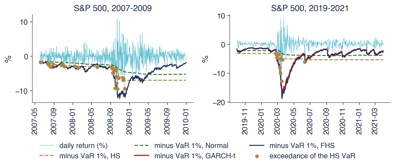




 SFM_ch10_var_methods