Bucharest University of Economic Studies IDA Institute Digital Assets Blockchain Research Center AI4EFin Artificial Intelligence for Energy Finance Romanian Academy, Institute for Economic Forecasting MSCA Digital Finance
Question: can flexible prediction methods forecast financial risk and returns better than the models of Chapters 7–10, and how do we check it honestly?
machine learning (ML): algorithms that learn a prediction rule from data, judged by their accuracy on new data
Route of the chapter
prediction against inference; overfitting, bias and variance; validation for time series without look-ahead bias
ridge and lasso; trees, random forest, gradient boosting; neural networks and the neural-network ARCH of the textbook
three applications: realised volatility, the sign of returns, VaR 1%; data snooping; a landmark paper
There are two cultures in the use of statistical modeling to reach conclusions from data. One assumes that the data are generated by a given stochastic data model. The other uses algorithmic models and treats the data mechanism as unknown.
The previous chapters built statistical models with a structure fixed in advance: distributions for returns, GARCH (generalised autoregressive conditional heteroskedasticity) models for volatility, models for VaR (value at risk). Machine learning (ML) starts from the opposite direction: it picks a flexible prediction rule from the data and judges it by its accuracy on data it has not seen. The question of the chapter is whether these methods forecast financial risk and returns better than the models of Chapters 7–10, and how such a gain is checked honestly.
The answer depends on the target. For the weekly volatility of the S&P 500, the lasso and a small neural network reduce the squared forecast error by 7.1% and 8.3% relative to the HAR (heterogeneous autoregressive) model, and the differences are significant. For Bitcoin, no model beats HAR. For the sign of tomorrow's return, no model is significantly better than the rule "always up", on any market studied. For VaR 1%, a linear quantile regression has the right violation rate on the S&P 500, while its flexible version runs short of data in the tail.
The difference between a real result and an apparent one lies in validation. A random split of the data produces an \(R^2\) of 34.5% for a simulated random walk, which has nothing to predict; a walk-forward scheme gives a negative \(R^2\) for the same data. The chapter therefore builds, before the models, the rules of evaluation: samples separated in time, simple benchmarks, tests of the difference between forecasts and a correction for the number of models tried.
Annualised realised volatility of the S&P 500 over the next 5 days and the HAR, random forest and MLP (multilayer perceptron) forecasts made at each day's close, in 2020 and 2025.
Learning outcomes
Explain the difference between prediction and inference, and the bias–variance trade-off.
Build a walk-forward evaluation with purging and recognise look-ahead bias and leakage.
Estimate ridge, the lasso, a regression tree, a random forest, gradient boosting and a small neural network.
Compare forecasts by out-of-sample \(R^2\), QLIKE and the Diebold–Mariano test, against a suitable benchmark.
Forecast VaR 1% by quantile regression and correct a Sharpe ratio for the number of strategies tried.
SummaryThe main ideas, the formulas and self-check questions.
The Contribution of Machine Learning to Statistics
The section places machine learning in the history of statistics. It starts from the perceptron of 1958, presents Breiman's distinction between data modelling and algorithmic modelling, separates prediction from inference and fixes the notation of supervised learning: features, target, loss function and hyperparameters. It ends with a map of the areas of finance where these methods help and those where they struggle.
Rosenblatt (1958) described a machine that learns to classify images by adjusting its weights after each error. The perceptron receives a vector of inputs \(x\), in the original version the signals of photocells, and outputs 1 if \(w_0 + w^\top x > 0\) and 0 otherwise. The weights \(w\) and the threshold \(w_0\) are not fixed by the designer but learned from examples: when the machine makes a mistake, the weights move in the direction that would have corrected it.
The Mark I Perceptron, built at Cornell in 1960, had 400 photocells, and its weights were set by electric motors. The central idea outlived this mechanical implementation: a linear decision rule, with parameters estimated by repeatedly correcting errors, is the ancestor of the neuron in the modern networks presented in Section 6.
Three later milestones mark the development of the field. In 1986, Rumelhart, Hinton & Williams (1986) showed how back-propagation of the error trains networks with hidden layers. In 2001 came random forests (Breiman, 2001b) and gradient boosting (Friedman, 2001), the tree methods used in Section 5. In 2024, the Nobel Prize in Physics was awarded to Hopfield and Hinton for their contributions to neural networks.
In brief
Rosenblatt (1958): a machine that learns to classify images by adjusting weights after each error
the perceptron: output \(1\) if \(w_0 + w^\top x > 0\), else \(0\)
\(x\): the inputs (photocell signals); \(w\): their weights, learned from examples; \(w_0\): the threshold term; \(w^\top x = \sum_j w_jx_j\)
the Mark I Perceptron (Cornell, 1960): 400 photocells, weights set by electric motors
Breiman (2001a), a statistician at Berkeley, describes two ways of using data. In the data-modelling culture, the researcher assumes a stochastic model, for example the linear regression \(y = x^\top\beta + \varepsilon\) or a GARCH model, estimates it and tests its parameters. The conclusions concern the parameters, and their validity depends on the assumed model being right.
In the algorithmic-modelling culture, the mechanism that generated the data is treated as unknown. The goal is a rule \(\hat f\) that predicts \(y\) well on new data, and a rule is judged by its prediction error, not by the plausibility of a model. Trees, random forests and neural networks belong to this culture.
The course has so far worked in the first culture, from Chapter 2 to Chapter 11: distributions, volatility models, tests of long memory. This chapter adds the second culture and asks under what conditions it brings a real gain on financial data, where noise is large and only one history is available.
In brief
Breiman (2001a), a statistician at Berkeley, describes two cultures
data modelling: assume a stochastic model (the linear regression \(y = x^\top\beta + \varepsilon\), GARCH), estimate it, test its parameters
algorithmic modelling: treat the mechanism as unknown; find a rule \(\hat f\) that predicts \(y\) well on new data
This course used the first culture in Chapters 2–11
this chapter adds the second, and asks when it pays off in finance
Inference asks whether a coefficient \(\beta_j\) differs from zero and how large the effect is, using standard errors and tests, as in Chapter 6. An example from the course is the leverage effect: the asymmetry parameter of a GJR-GARCH (Glosten–Jagannathan–Runkle GARCH) model, from Chapter 9, says whether price falls raise volatility more than rises.
Prediction asks how close the forecast \(\hat y\) is to the value \(y\) on data the model has never seen. Typical examples are next week's volatility and tomorrow's VaR 1%. The coefficients of a prediction model may be hard to interpret, and sometimes do not even exist as parameters with an economic meaning; only the error on new data matters.
The two goals can conflict. A biased estimator, such as ridge or the lasso of Section 4, can have a smaller prediction error than the unbiased OLS (ordinary least squares) estimator, because it gains more by reducing variance than it loses through bias. Conversely, a model that predicts well does not prove a causal mechanism: it may exploit a stable correlation without saying anything about its cause.
In brief
Inference: is \(\beta_j \ne 0\)? how large is the effect? (standard errors, tests, Chapter 6)
example: does the leverage effect exist (GJR-GARCH, Chapter 9)?
Prediction: how close is \(\hat y\) to \(y\) on data the model has never seen?
example: next week's volatility; tomorrow's VaR 1%
the coefficients may be uninterpretable; what matters is the error on new data
The two goals can conflict
a biased estimator (ridge, lasso) can predict better than the unbiased OLS
a model that predicts well does not prove a causal mechanism
Supervised learning starts from pairs \((x_t, y_t)\),\(t = 1, \dots, n\), where \(t\) indexes the observations, for example days or weeks. The vector \(x_t \in \mathbb{R}^p\) contains the features: \(p\) numbers known at time \(t\), such as past volatilities and returns. The target \(y_t\) is the quantity we want to forecast, for example next week's volatility.
The condition "known at time \(t\)" is essential in finance. A feature that uses, even indirectly, information from after time \(t\) makes the forecast look better than it could be in real time; Section 3 treats this error in detail.
Problems are divided by the nature of the target. In regression, \(y\) is a continuous variable, for example a volatility or a return. In classification, \(y\) is a class: up or down, default or repayment, as in the scoring models of Chapter 12. The methods of the chapter have versions for both types of problem.
In brief
Data \((x_t, y_t)\), \(t = 1, \dots, n\)
\(t\): the index of the observation (a day, a week); \(n\): the number of observations
\(x_t \in \mathbb{R}^p\): the features, \(p\) numbers known at time \(t\) (past volatilities, past returns)
\(y_t\): the target, the quantity we want to forecast (next week's volatility)
Two types of problems
regression: \(y\) continuous (volatility, return)
classification: \(y\) a class (up/down, default; Chapter 12)
Learning means choosing, from a family of candidate rules \(\mathcal{F}\), the rule \(\hat f\) that minimises the average loss \(\frac1n\sum_t L(y_t, f(x_t))\). The loss function \(L(y, \hat y)\) gives the cost of the forecast \(\hat y\) when \(y\) is observed. The family \(\mathcal{F}\) may be, for example, the set of all linear regressions or of all trees of depth 3; the richer the family, the more closely the chosen rule can adapt to the data.
The loss function must match the purpose of the forecast. The squared error \((y - \hat y)^2\), whose average is the MSE (mean squared error), is the default choice for regression. For variances, the course used QLIKE from Chapter 8; for VaR, the quantile (pinball) loss from Chapter 10; for probabilities, the log loss from Chapter 12.
The parameters of a rule, such as coefficients or weights, are learned by estimation. A hyperparameter is chosen before estimation and controls the complexity of the rule: the depth of a tree, the penalty \(\lambda\) in ridge regression, the number of neurons in a network. Choosing hyperparameters is itself a form of estimation and needs separate data, as the following sections show.
In brief
Learning = choose \(\hat f\) in a family \(\mathcal{F}\) that minimises the average loss\(\frac1n\sum_t L(y_t, f(x_t))\)
\(f(x_t)\): the forecast of a rule \(f\) for observation \(t\); \(L(y, \hat y)\): the cost of forecasting \(\hat y\) when \(y\) is observed
\(\mathcal{F}\): the candidate rules (all linear regressions, all trees of depth 3); \(\hat f\): the rule chosen from the data
Losses used in this course
squared error \((y - \hat y)^2\) (MSE: mean squared error); QLIKE for variances (Chapter 8)
quantile (pinball) loss for VaR (Chapter 10); log loss for probabilities (Chapter 12)
A hyperparameter is chosen before the fit
examples: tree depth, penalty \(\lambda\), number of neurons
the parameters (coefficients, weights) are learned by the fit
Strengths and Limitations of Machine Learning in Finance
Machine learning has a chance of success when the target has structure and the data are sufficient. Volatility is such a case: Chapters 8 and 9 showed that it is persistent, so much of it can be forecast, and nonlinear effects are plausible. A second case is cross-sections with thousands of stocks and many characteristics, as in the case study of Section 11.
The main difficulty is a low signal-to-noise ratio. Daily returns are almost unpredictable (Chapter 7), and a flexible model applied to them mostly learns noise. Markets change regimes, and crises bring situations absent from the training history, so the past is an imperfect training set for the future.
There is also a limit of principle: we have a single price history. The experiment cannot be repeated, the observations are dependent over time, and the real number of independent episodes, for example of crises, is small. These features explain why validation takes as important a place in the chapter as the models.
In brief
Helps: targets with structure and enough data
volatility is persistent (Chapters 8–9): a lot to predict, nonlinear effects possible
cross-sections with thousands of stocks and many characteristics (the case study)
Struggles: a low signal-to-noise ratio
daily returns are close to unpredictable (Chapter 7): a flexible model fits the noise
markets change (regimes, crises): the past is an imperfect training set
one price history: we cannot repeat the experiment, and the observations are dependent
Section summary
Machine learning adds to statistics the culture of algorithmic modelling: a prediction rule chosen from the data and judged by its error on new data. The ingredients are the features, the target, the loss function and the hyperparameters. In finance, the approach has a chance where the target has structure, as volatility does, and struggles where noise dominates, as with daily returns. The next section explains why flexibility has a cost.
Overfitting, Bias and Variance
The section shows why a more flexible model is not automatically a better model. It distinguishes training error from test error, derives the decomposition of test error into bias, variance and noise, and illustrates the trade-off between them by a simulation with regression trees of different depths.
The training error is the average loss on the data used for estimation; the test error is the average loss on new data generated by the same process. The first always falls when the model becomes more flexible, because a richer family of rules also contains the simpler rules. Training error therefore cannot be used to compare models of different complexity.
Overfitting occurs when the model learns, besides the signal, the noise of the training sample. The symptom is a small training error together with a large test error. The extreme case is a tree with one leaf per observation: it reproduces the training data exactly, so its training error is zero, but its forecasts for new observations are poor.
Underfitting is the opposite error: the model is too rigid to capture the signal. An example is a constant volatility forecast in a market with volatility clustering: it ignores exactly the structure that makes volatility predictable.
In brief
Training error: the average loss on the data used for the fit; test error: on new data from the same process
the training error always falls as the model becomes more flexible
Overfitting: the model learns the noise of the training sample
symptom: a small training error and a large test error
a tree with one leaf per observation has zero training error and predicts badly
Underfitting: the model is too rigid to capture the signal
example: a constant forecast of volatility in a world with volatility clustering
Assume the data are generated by \(y = f(x) + \varepsilon\), with \(E[\varepsilon] = 0\) and \(\mathrm{Var}(\varepsilon) = \sigma^2\). The function \(f\) is the true, unknown relation between \(x\) and \(y\), and \(\varepsilon\) is the noise, unpredictable from \(x\). The estimate \(\hat f\) is obtained on a random training sample; another sample would give another estimate, so \(\hat f(x_0)\) is a random variable.
For a new point \(x_0\), with \(y_0 = f(x_0) + \varepsilon_0\), the expected test error splits into three terms:
The expectation is taken over all possible training samples and over the noise \(\varepsilon_0\). The first term is the squared bias: the distance between the average estimate and the true value. The second is the variance: how much \(\hat f(x_0)\) changes from one sample to another. The third is the noise, which does not depend on the model.
The derivation starts by writing the error at \(x_0\) as a sum of three terms: \(y_0 - \hat f = (f - E\hat f) + (E\hat f - \hat f) + \varepsilon_0\). Squaring and taking expectations, the three squares give the squared bias, the variance and \(\sigma^2\). The cross terms have mean zero: the first term is a constant, \(E[E\hat f - \hat f] = 0\), and \(\varepsilon_0\) is independent of the training sample.
The decomposition (13.1) explains the bias–variance trade-off. A rigid model has large bias and small variance: it gives almost the same forecast on any sample, but a systematically wrong one. A flexible model has small bias and large variance: it fits well on average, but its forecast depends strongly on the particular sample. The optimal complexity balances the two terms.
The third term, \(\sigma^2\), is a floor: no model goes below it. For daily returns, \(\sigma^2\) is almost all of the error, because the predictable part \(f(x)\) is very small. In this situation, any extra variance brought by a flexible model shows up directly in the test error, and the possible gain from reducing bias is small.
In brief
Derivation: write \(y_0 - \hat f = (f - E\hat f) + (E\hat f - \hat f) + \varepsilon_0\), all at \(x_0\)
square and take the expectation: the three squares give bias\(^2\), variance and \(\sigma^2\)
the cross terms have mean 0: \(E[E\hat f - \hat f] = 0\), and \(\varepsilon_0\) is independent of the training sample
Reading the decomposition
a rigid model: large bias, small variance
a flexible model: small bias, large variance
\(\sigma^2\) is the floor: no model goes below it; in daily returns \(\sigma^2\) is almost everything
Question for the room With noise variance σ² = 0.04 instead of 0.09 (extra run), at which depth is the expected test error lowest?
Answer
At depth 4 (0.063), against depth 3 (0.132) with σ² = 0.09. With less noise the variance of deep trees costs less, so the optimum moves to a more flexible model; with σ² = 0.25 the minimum stays at depth 3 (0.329).
The simulation makes the decomposition visible. The data are generated by \(y = \sin(2\pi x) + \varepsilon\), with noise variance \(\sigma^2 = 0.09\) and \(n = 80\) observations, and the experiment is repeated on 300 training samples. The left panel shows a single sample and the trees of depth 1, 3 and 10 estimated on it; regression trees are defined in Section 5.
The depth-1 tree has a single split and cannot follow the shape of the sine wave: its squared bias is 0.070 and its variance 0.031. The depth-10 tree follows every point: its squared bias is practically zero (0.000), but its variance rises to 0.090, as large as the noise variance. Between the two extremes, the test error is lowest at depth 3, at 0.132.
The minimum, 0.132, is only a little above the floor \(\sigma^2 = 0.09\): in this simulation the signal is strong, and a model of medium complexity captures it almost completely. The chart shows the three components of (13.1) as functions of depth and the U shape of the test error that results from their sum.
In brief
Simulation: \(y = \sin(2\pi x) + \varepsilon\), \(\sigma^2 = 0.09\), \(n = 80\), 300 training samples; left: one sample with trees of depth 1, 3 and 10
Depth 1: bias\(^2\)\(0.070\), variance \(0.031\); depth 10: bias\(^2\)\(0.000\), variance \(0.090\); the test error is smallest at depth 3 (\(0.132\))
As depth increases, the training error falls from 0.172 to 0.002. The test error falls at first, while the reduction in bias dominates, and then rises, when the increase in variance becomes more important. The depth-10 tree has a training error close to zero and a test error of 0.180, larger than that of the depth-3 tree.
The practical consequence is that a model is never chosen by its training error: that would always favour the most flexible model. Complexity is a hyperparameter and must be chosen on data that were not used to estimate the parameters.
In finance, noise is much larger relative to signal than in this simulation. The minimum of the U curve then moves towards simpler models, so the best model is usually simpler than the depth-3 tree of the example.
In brief
The training error falls from \(0.172\) to \(0.002\); the test error falls, then rises
depth 10 has almost zero training error and a test error of \(0.180\), worse than depth 3
Consequences for practice
never select a model by its training error
complexity is a hyperparameter: choose it on data that were not used for the fit
in finance the noise is large, so the best model is usually simpler than in this simulation
Section summary
Test error splits into squared bias, variance and noise, (13.1). Flexibility reduces bias and increases variance, hence the U shape of the test error, and the noise sets a floor that no model goes below. Complexity is therefore chosen on data not used for estimation, which requires a validation scheme suited to time series, the subject of the next section.
Validation for Time Series
The section sets the rules by which all the models of the chapter are evaluated. It defines the roles of the training, validation and test samples, the two errors that make a model look better than it is, look-ahead bias and leakage, and the validation schemes suited to time series. An experiment with a simulated random walk shows how large the effect of a wrong scheme can be.
Data have three roles. The training sample is used to estimate the parameters of each candidate model. The validation sample is used to choose the hyperparameters and the model. The test sample is used for a single measurement of the error of the finally chosen model; only this measurement honestly estimates performance on new data.
Any decision taken on the basis of the test sample turns it into a validation sample. Trying ten models on the test data and reporting the best is no longer testing but model selection, and the reported error is optimistic. Section 10 quantifies this optimism for Sharpe ratios.
K-fold cross-validation (CV) splits the data into \(K\) parts; each part is in turn the validation set, and the other \(K - 1\) parts train the model. The scheme is valid for i.i.d. data. For time series, Bergmeir, Hyndman & Koo (2018) show that it remains valid only under strict conditions, when no dependence is left in the model's errors.
In brief
Three roles for the data
training: estimate the parameters of each candidate model
validation: choose the hyperparameters and the model
test: measure the error of the final choice, once
Every look at the test sample turns it into a validation sample
trying ten models on the test data and reporting the best is model selection, not testing
K-fold cross-validation: split the data into \(K\) folds; each fold is the validation set once, the others train the model
valid for i.i.d. data; for a time series only under strong conditions (no dependence left in the errors) Bergmeir, Hyndman & Koo (2018)
Look-ahead bias occurs when the forecast for day \(t\) uses information that was not available at the close of day \(t - 1\). The usual sources are features computed with future prices, for example a centred moving average or a full-sample mean, scaling or standardisation with full-sample statistics, data revised later, and using today's index membership for the past (survivorship).
Leakage is a related error: information about the test target reaches the training sample. The typical case is overlapping targets. The 21-day return starting on day \(t\) and the one starting on day \(t + 1\) share 20 days. If a random split puts day \(t + 1\) in training and day \(t\) in the test set, the model has seen almost all of the answer before being tested.
Both errors make a model look better than it can be in real time, and neither shows up in the training error or in code that runs without errors. They must be ruled out by the construction of the validation scheme, not discovered afterwards.
In brief
Look-ahead bias: the forecast for day \(t\) uses information that was not available at the close of day \(t - 1\)
features computed with future prices (a centred moving average, a full-sample mean)
scaling or standardising with statistics of the whole sample; revised data; today's index members (survivorship)
Leakage: information about the test target reaches the training sample
overlapping targets: the 21-day return from day \(t\) and from day \(t + 1\) share 20 days
a random fold puts day \(t + 1\) in training and day \(t\) in test: the model has seen the answer
Both make a model look better than it can be in real time
Question for the room With a 22-day target (h = 22, extra run), how many training days does the 2013 fold have?
Answer
1,171: the purging removes 22 rows instead of 5, so 17 fewer than the 1,188 days with h = 5; the last training day becomes 28 November 2012. The test remains the 252 days of 2013.
Question for the room Random K-fold, fold 1 (K = 5): of its 12 test observations, how many have at least one neighbour (the day before or the day after) in training?
Answer
11 of 12. A random fold scatters the test days among the training days, and with overlapping targets the neighbour has almost the same target: the model has practically seen the answer. With K = 8 it is the same, 7 of 8.
The chart compares three schemes. Walk-forward validation trains the model on the past, tests it on the next block and then moves forward. In the expanding-window version, each step keeps the whole past in the training sample. The scheme mimics exactly the situation of an analyst forecasting in real time.
The second scheme is K-fold with purging and embargo, proposed by López de Prado (2018). Test blocks may also lie in the middle of the sample, but the training rows whose targets overlap the test block are removed (purging), together with a few rows after it (embargo). In this way, no training target contains information from the test period.
The third scheme, random K-fold, appears in the chart as a point of comparison: it shuffles the days and ignores time order. The experiment on the following slides shows what this scheme produces on overlapping targets.
In brief
Walk-forward: train on the past, test on the next block, move forward; the expanding window keeps all the past
Purged K-fold with embargoLópez de Prado (2018): drop the training rows whose targets overlap the test block (purging) and a few rows after it (embargo)
For the S&P 500, the chapter uses data starting on 8 April 2008 and one fold for each calendar year from 2013, 14 folds in all. The model is re-estimated every January on all previous days, with an expanding window, and tested on every day of that year.
The target is the average variance over the next 5 days, so the last rows before the test year have targets that end in that year. Purging removes them: for 2013 the last 5 training rows, from 24 December 2012, are dropped from training. The 2013 fold thus trains on 1,188 days and tests on 252, and the 2026 fold trains on 4,458 days.
Hyperparameters are chosen inside each training window, by a walk-forward split of the training data only; the test year influences no choice. No embargo is needed, because the test block always comes after the training block and there are no training rows after the test period.
In brief
The design used in this chapter for the S&P 500 (data from 8 April 2008)
one fold per calendar year from 2013: 14 folds; the model is re-estimated each January
training window: all earlier days (expanding); test: every day of the year
Purging: the target is the mean variance of the next 5 days
for 2013 the last 5 training rows (from 24 December 2012) are dropped: their targets reach into 2013
the 2013 fold trains on 1 188 days and tests on 252; the 2026 fold trains on 4 458 days
Inside each training window, hyperparameters are tuned by a walk-forward split of the training data only
no embargo is needed: the test block always comes after the training block
Leakage in Practice: Random Folds on Overlapping Targets
Question for the room With a 5-day target instead of 21 (extra run), what R² does random K-fold report for the simulated random walk?
Answer
17.8%, against 34.5% with 21 days: the targets of two neighbouring days now share 4 of 5 returns, not 20 of 21, so the leakage is smaller but still large. Walk-forward stays negative (−17.5%); with 63 days random K-fold rises to 35.8%.
The experiment uses a random forest for the return over the next 21 days, with features built from past returns and volatilities. Performance is measured by the out-of-sample \(R^2\) relative to the training mean, defined in Section 7: a positive value means a smaller squared error than the mean, a negative one a larger error.
The first data set is a simulated random walk, in which future returns are independent of the past. Random 5-fold validation reports an \(R^2\) of 34.5%, and walk-forward validation an \(R^2\) of −26.1%. On the S&P 500, with 6,631 days, the two values are 36.9% and −38.0%.
The results on real data are almost identical to those on the random walk. The similarity shows that the large \(R^2\) of the random folds reflects not a predictability of the S&P 500 but the validation scheme.
In brief
Random forest for the next 21-day return from past returns and volatilities; out-of-sample \(R^2\) against the training mean
Simulated random walk: random 5-fold \(34.5\%\), walk-forward \(-26.1\%\); S&P 500 (6 631 days): \(36.9\%\) and \(-38.0\%\)
The random walk has nothing to predict, yet the random folds report an \(R^2\) of 34.5%. The explanation is leakage: the random forest memorises neighbouring days in the training set, whose targets share 20 of 21 returns with the test day. The forecast "guesses" the target because it has already seen almost all of it.
Walk-forward validation gives a negative \(R^2\): the random forest learns the noise of the training years and does worse than the simple training mean. Purging, that is removing 21 days at the boundary between training and test, changes the result little, because in walk-forward only the rows at the boundary have targets overlapping the test period.
The resulting rule is simple: with overlapping targets or dependent data, time order is never shuffled. A large \(R^2\) obtained with random folds on such data says nothing about the forecasting ability of the model.
In brief
The random walk has nothing to predict, yet random folds report \(R^2 = 34.5\%\)
the forest memorises neighbouring days, whose targets share 20 of 21 returns with the test day
Walk-forward gives a negative \(R^2\): the forest fits noise and loses against the training mean
purging (a gap of 21 days) changes little here, because in walk-forward only the boundary rows overlap
Rule: with overlapping targets or dependent data, never shuffle the time order
Section summary
Data have three roles, training, validation and test, and the test sample is used once. Look-ahead bias and leakage make a model look better than it can be in real time; on overlapping targets, random folds give an \(R^2\) above 30% even for pure noise. All the empirical results of the chapter therefore use walk-forward validation with purging. The next section starts the series of models with penalised regression.
Penalised Regression: Ridge and Lasso
The section starts from the instability of the OLS estimator when features are many and correlated. It introduces ridge regression and the lasso, which add a penalty on the coefficients, computes them in an example with a single feature and applies them to the volatility features of the S&P 500.
where \(X\) is the \(n \times p\) matrix whose row \(t\) is \(x_t^\top\), and \(y\) is the vector of targets. The estimator is unbiased, but its variance, \(\sigma^2(X^\top X)^{-1}\), with \(\sigma^2\) the error variance, becomes very large when the features are many or strongly correlated, because the matrix \(X^\top X\) becomes nearly singular.
Volatility features are a typical example: today's realised variance, this week's and this month's move together. OLS can then produce large coefficients of opposite signs that offset each other in sample; out of sample, where the correlations change slightly, the offsetting no longer works and the forecasts deteriorate.
Penalised regression minimises the squared error plus a penalty on the size of \(\beta\). The penalty introduces a bias towards zero but reduces the variance of the estimator. In terms of the decomposition (13.1), a small bias is accepted for a large reduction in variance.
\(X\): the \(n \times p\) matrix whose row \(t\) is \(x_t^\top\); \(y\): the vector of targets; \(\arg\min_\beta\): the \(\beta\) that minimises the sum
unbiased, but its variance \(\sigma^2(X^\top X)^{-1}\) (\(\sigma^2\): the error variance) explodes when features are many or strongly correlated
Volatility features are highly correlated: today's, this week's and this month's realised variance
OLS may give large coefficients of opposite signs that cancel in sample and fail out of sample
Penalised regression: minimise the squared error plus a penalty on the size of \(\beta\)
accept a little bias for a large reduction in variance (the trade-off of Section 2)
The term \(\sum_j \beta_j^2\) is large when the coefficients are large, and \(\lambda \ge 0\) sets the strength of the penalty; \(I\) is the \(p \times p\) identity matrix. For \(\lambda = 0\) we obtain OLS, and for \(\lambda \to \infty\) all coefficients tend to zero. The parameter \(\lambda\) is a hyperparameter and is chosen by validation.
The closed form in (13.2) has an important consequence. The matrix \(X^\top X + \lambda I\) is invertible for any \(\lambda > 0\), even if \(X^\top X\) is not. Ridge therefore works even when there are more features than observations, a situation in which OLS has no unique solution.
In brief
Hoerl & Kennard (1970): minimise the squared error plus a penalty on the squared coefficients
\[ \hat\beta^{\,ridge} = \arg\min_\beta \sum_t (y_t - x_t^\top\beta)^2 + \lambda\sum_j \beta_j^2 = (X^\top X + \lambda I)^{-1}X^\top y \]
Notation
\(\beta_j\): the coefficient of feature \(j\); \(\sum_j \beta_j^2\): the penalty term, large when the coefficients are large
\(\lambda \ge 0\): the strength of the penalty; \(\lambda = 0\) gives OLS, \(\lambda \to \infty\) gives \(\hat\beta \to 0\)
\(I\): the \(p \times p\) identity matrix
Consequence
\(X^\top X + \lambda I\) is always invertible for \(\lambda > 0\): ridge works even with more features than observations
The factor \(S_{xx}/(S_{xx} + \lambda)\) lies in the interval \((0, 1]\) and is the fraction of the OLS coefficient that ridge keeps. Shrinkage is stronger when \(\lambda\) is large relative to \(S_{xx}\), that is, when the feature carries little information.
In the example on the slide, \(S_{xx} = 100\) and \(S_{xy} = 30\). The OLS coefficient is \(30/100 = 0.30\), and the ridge coefficient with \(\lambda = 50\) is \(30/150 = 0.20\), with a shrinkage factor of 0.67. Ridge shrinks all coefficients towards zero but sets none of them exactly to zero: for any finite \(\lambda\), the factor stays positive.
The absolute value has a kink at zero, and the solution can stop at this point: some coefficients become exactly zero. Besides shrinkage, the lasso thus performs variable selection.
For a single feature, the solution is soft thresholding: \(\hat\beta^{\,lasso} = \mathrm{sign}(S_{xy})\,\max(|S_{xy}| - \lambda/2,\, 0)/S_{xx}\), where \(\mathrm{sign}(S_{xy})\) is the sign, \(+1\) or \(-1\). If \(|S_{xy}| \le \lambda/2\), the coefficient is exactly zero. With the same data as for ridge and \(\lambda = 20\), the coefficient is \((30 - 10)/100 = 0.20\); for \(\lambda \ge 60\) the feature leaves the model.
In practice, the features are standardised before estimation, because the penalty depends on their units; the mean and standard deviation used for standardisation are computed on the training data only, otherwise look-ahead bias appears. The parameter \(\lambda\) is chosen by walk-forward cross-validation. The elastic net combines the two penalties, \(L_1\) and \(L_2\).
Question for the room ▶ raises λ from 50 to 200. What is the ridge β̂ now?
Answer
0.10 = 30/(100 + 200); the shrinkage factor falls from 0.67 to 0.33. The coefficient approaches zero but is not zero for any finite λ; the lasso with λ = 200 is already 0.
Question for the room ▶ raises λ from 20 to 60. What is the lasso β̂ now?
Answer
Exactly 0: λ/2 = 30 = |S_xy|, so max(30 − 30, 0) = 0, and it stays 0 for any λ ≥ 60. Ridge with the same λ would give 30/160 = 0.19.
Question for the room ▶ raises the lasso penalty up to λ = 1. Which feature is the last with a non-zero coefficient?
Answer
Log RV week: it stays non-zero up to λ = 0.86 on the grid, after log RV month (0.46), log RV day (0.21) and the negative return (0.18). On its own, the weekly variance is the most informative feature; ridge, on the left, sets no coefficient to zero.
The chart shows the coefficient paths as functions of \(\lambda\) for a real problem. The target is the log of the average variance proxy over the next 5 days for the S&P 500, in 2008–2012 (1,193 days), and the features are the 11 standardised features of Section 7. For large \(\lambda\) all coefficients are close to zero; as \(\lambda\) falls, they approach the OLS values.
The value chosen by walk-forward cross-validation is \(\lambda = 0.0079\). At this value, the lasso keeps 10 of the 11 features; the absolute return leaves the model. The coefficient on the weekly variance rises from +0.199 in OLS to +0.283 in the lasso.
The rise of the weekly coefficient seems to contradict the idea of shrinkage, but it is explained by correlations. When a correlated feature leaves the model or is shrunk, part of its weight passes to the remaining features. Shrinkage concerns the norm of the coefficient vector, not each coefficient separately.
Three of the features are exactly collinear: the absolute return is \(|r| = r - 2\min(r, 0)\), so the matrix of the 11 features has rank 10. OLS therefore has no unique solution for the coefficients of \(r\),\(\min(r, 0)\) and \(|r|\): any shift along the direction of this identity leaves the fit unchanged, and the values reported are the minimum-norm solution. The coefficients of the other eight features, including the weekly one, are unique. The lasso resolves the ambiguity in its own way, by setting the coefficient of \(|r|\) to zero.
In brief
Target: log of the mean variance proxy of the next 5 days, S&P 500, 2008–2012 (1 193 days); 11 standardised features (Section 7)
Lasso with \(\lambda = 0.0079\) (walk-forward CV): 10 of 11 features kept; the week coefficient rises from \(+0.199\) (OLS) to \(+0.283\), the absolute return drops out
The design is exactly collinear, \(|r| = r - 2\min(r, 0)\) (rank 10): the OLS coefficients of \(r\), \(\min(r,0)\), \(|r|\) are not unique (shown: the minimum-norm solution); the others are unique
In the left panel, ridge shrinks all coefficients smoothly and together, and correlated features share their weight. The negative return keeps its negative sign to the end: market falls raise future volatility, which corresponds to the leverage effect of Chapter 9.
In the right panel, the lasso brings in the features one at a time as \(\lambda\) falls. The weekly variance enters first, because it is the most informative feature on its own. At the chosen value of \(\lambda\), the lasso keeps the HAR structure, with daily, weekly and monthly components, plus the negative return, with coefficient −0.112.
The lasso selects features but does not test them. A coefficient equal to zero is not the equivalent of a large p-value: it only shows that, at this \(\lambda\), the feature does not improve the forecast enough to pay for its penalty. Among strongly correlated features, the lasso's choice can be unstable from one sample to another.
In brief
Ridge (left): all coefficients shrink smoothly and together; correlated features share the weight
the negative return keeps a negative sign until the end: falling markets raise future volatility (the leverage effect, Chapter 9)
Lasso (right): the features enter one by one as \(\lambda\) falls
the weekly variance enters first: the most informative single feature
at the chosen \(\lambda\) the lasso keeps the HAR structure (day, week, month) plus the negative return, \(-0.112\)
The lasso selects; it does not test: a zero coefficient is not a p-value
Section summary
Ridge, (13.2), and the lasso stabilise regression by penalising the coefficients: ridge shrinks all coefficients without setting any to zero, while the lasso sets some of them exactly to zero. On the volatility features of the S&P 500, the lasso recovers the HAR structure plus the leverage effect. Both remain linear models; the next section turns to trees, which capture nonlinearities and interactions.
Trees, Random Forest and Gradient Boosting
The section builds regression trees, from the splitting rule to an example computed by hand and a tree estimated on S&P 500 volatility. It then shows the two ways of combining trees, the averaging of a random forest and the sequence of gradient boosting, and compares them on the volatility data.
A regression tree splits the feature space into rectangles and predicts, in each rectangle, the mean of \(y\) within it. The final rectangles are called leaves. Each split uses a feature \(j\) and a threshold \(s\): observations with \(x_j \le s\) go to the left, those with \(x_j > s\) to the right.
The tree is estimated greedily: at each node, the pair \((j, s)\) is chosen that minimises the sum of squared errors (SSE),
where \(\bar y_L\) and \(\bar y_R\) are the means of \(y\) in the two groups, that is, the two forecasts. The procedure is repeated in each half until a stopping rule is met, for example a maximum depth or a minimum number of observations in a leaf.
Trees capture nonlinear effects and interactions without these being specified in advance, and they are insensitive to monotone transformations of the features, since they depend only on the order of the values. Their weak point is high variance: a small change in the data can change the first split and, through it, the whole tree, as in the simulation of Section 2.
In brief
A regression tree splits the feature space into rectangles and predicts the mean of \(y\) in each leaf
split rule: a feature \(j\) and a threshold \(s\): left \(x_j \le s\), right \(x_j > s\)
Greedy fit: at each node choose \((j, s)\) that minimises \(\mathrm{SSE} = \sum_{\text{left}}(y - \bar y_L)^2 + \sum_{\text{right}}(y - \bar y_R)^2\)
SSE: sum of squared errors; \(\bar y_L\), \(\bar y_R\): the means of \(y\) in the left and right groups (the two forecasts)
repeat in each half until a stopping rule: maximum depth, minimum number of observations per leaf
Strengths and weaknesses
nonlinear effects and interactions without specifying them; insensitive to monotone transformations of \(x\)
high variance: a small change in the data can change the whole tree (Section 2)
The example uses six weeks. The feature \(x\) is this week's volatility, in percent, with values 0.6, 0.8, 1.0, 1.5, 2.0, 2.4, and the target \(y\) is next week's volatility, with values 0.7, 0.9, 0.8, 1.6, 2.1, 2.2. Without any split, the forecast is the mean \(\bar y = 1.38\), and the SSE is 2.268.
The candidate thresholds are the midpoints between consecutive values of \(x\): 0.70, 0.90, 1.25, 1.75, 2.20. For each threshold, the two means and the SSE are computed. The threshold 0.70 leaves a single observation on the left and gives an SSE of 1.708; the threshold 1.25 separates the first three weeks from the last three, with leaves 0.80 and 1.97 and an SSE of 0.227, the smallest value in the table.
The best split is therefore \(s = 1.25\). It explains \(1 - 0.227/2.268 = 0.90\) of the variation of the target: a single question, "is current volatility above 1.25%?", separates calm weeks from turbulent ones. A deeper tree would repeat the same search in each of the two groups.
In brief
\(s\)
\(\bar y_L\)
\(\bar y_R\)
SSE
\(0.70\)
\(0.70\)
\(1.52\)
\(1.708\)
\(0.90\)
\(0.80\)
\(1.68\)
\(1.248\)
\(1.25\)
\(0.80\)
\(1.97\)
\(0.227\)
\(1.75\)
\(1.00\)
\(2.15\)
\(0.505\)
\(2.20\)
\(1.22\)
\(2.20\)
\(1.468\)
Six weeks: \(x\) = this week's volatility (%), \(y\) = next week's
Question for the room What share of the variation does the threshold s = 1.75, the second best in the table, explain?
Answer
0.78 = 1 − 0.505/2.268, against 0.90 for s = 1.25. The threshold 1.75 moves the week with x = 1.5 (y = 1.6) into the left leaf, whose mean rises to 1.00 and whose deviations grow.
Question for the room ▶ moves to depth 3 (extra run). Do all splits still use log RV week?
Answer
No: 5 of the 6 splits use log RV week, one uses log RV month (≤ 0.069), in the branch with moderate weekly volatility. The first split stays log RV week ≤ 0.44, because a greedy tree does not revise its choices at the top.
The tree in the chart is estimated on the S&P 500 in 2008–2012, with target and features expressed as the log of variance (in %² per day). At each node, value is the mean of the target for the observations in that node, hence the tree's forecast if it stopped there.
The first split is "weekly log RV ≤ 0.44", where RV is realised variance. The threshold corresponds to an annual volatility of about 19.8%: the tree first separates the calm regime from the turbulent one. All splits use the weekly variance, the same feature the lasso picked first in Section 4.
The depth-2 tree has four leaves, hence four possible forecast levels. It is easy to read, but its forecast is a step function of current volatility; random forests and boosting, on the following slides, smooth these steps by combining many trees.
In brief
S&P 500, 2008–2012, target and features in log variance (%\(^2\) per day); value: the mean of the target in the node
Interpretation: the first split, log RV week \(\le 0.44\), is an annual volatility of about 19.8%; all splits use the weekly variance, the feature the lasso picked first
A random forest (Breiman, 2001b) averages \(B\) deep trees, each grown on a bootstrap sample of the training data, a method called bagging (bootstrap aggregating); the bootstrap was introduced in Chapter 2. In addition, only a random subset of features is tried at each split. This second source of randomness makes the trees less correlated with each other.
The effect of averaging is seen in a simple calculation. If each of the \(B\) trees has variance \(\sigma^2\) and the correlation between any two is \(\rho\), then
The second term falls with \(B\), the first does not. With \(\rho = 0.3\) and \(\sigma^2 = 1\), the variance is 1.000 for one tree, 0.370 for 10 trees and 0.302 for 300 trees, close to the floor \(\rho\sigma^2 = 0.3\).
Two practical conclusions follow from (13.3). More trees do not cause overfitting; they only bring the variance closer to the floor. The floor itself falls if the trees are less correlated, for example by trying fewer features at each split. The chapter uses 300 trees, at least 20 observations per leaf and half of the features tried at each split.
In brief
Breiman (2001b): average \(B\) deep trees, each grown on a bootstrap sample (Chapter 2) of the training data (bagging)
at each split only a random subset of the features is tried: the trees become less correlated
Why averaging works: \(B\) trees, each with variance \(\sigma^2\) and pairwise correlation \(\rho\)
\(\mathrm{Var}(\text{average}) = \rho\sigma^2 + (1 - \rho)\sigma^2/B\): the part \(\rho\sigma^2\), common to all trees, does not fall with \(B\)
Gradient boosting (Friedman, 2001) builds the model step by step, each new small tree learning what the earlier trees missed. It starts from the constant forecast \(F_0 = \bar y\). At step \(m\), a small tree \(h_m\) is fitted to the residuals \(y_t - F_{m-1}(x_t)\), and the model is updated:
where \(\nu\) is the learning rate. For squared loss, the residuals equal minus the gradient of the loss with respect to the forecast; hence the name of the method, which is gradient descent in the space of functions.
The two ensemble methods attack different terms of (13.1). A random forest uses deep trees, with small bias, in parallel, and averaging reduces their variance. Boosting uses small trees, with large bias, in sequence, and each step reduces the bias. This is why, in boosting, too many steps cause overfitting, while in a random forest they do not.
The method works with any differentiable loss, replacing the residuals by minus the gradient of that loss. With the quantile loss we obtain quantile gradient boosting, used for VaR in Section 9.
In brief
Friedman (2001): build the model step by step, each new small tree fitting what the previous ones missed
start with \(F_0 = \bar y\); at step \(m\), fit a shallow tree \(h_m\) to the residuals \(y_t - F_{m-1}(x_t)\)
update \(F_m = F_{m-1} + \nu\, h_m\), with the learning rate\(0 < \nu \le 1\)
for squared loss the residuals are minus the gradient of the loss: hence the name
Random forest against boosting
forest: deep trees in parallel, averaging reduces variance
boosting: shallow trees in sequence, each step reduces bias; too many steps overfit
Any differentiable loss works: quantile loss gives quantile boosting (Section 9)
One Tree, a Forest and Boosting on Volatility Data
Question for the room ▶ raises B from 10 to 300, with ρ = 0.3 and σ² = 1. What is the variance of the average now?
Answer
0.302 = 0.3 + 0.7/300, against 0.370 at B = 10. The shared part ρσ² = 0.3 does not vanish however many trees are added; the floor falls only if the trees become less correlated.
Worked example: boosting with depth-1 trees on the six weeks (extra computation)
Question for the room Extra computation, ν = 0.1: after how many steps does the training SSE fall below half of 2.268?
Answer
After 4 steps: the SSE falls to 1.880, 1.566, 1.312 and 1.101. Each step applies only ν = 10% of the tree fitted to the current residuals, so the error falls geometrically, not linearly. After 50 steps the SSE is 0.007: on the training data boosting gets close to zero, which is why the number of steps is chosen on validation data.
Question for the room ▶ reduces the forest to a single tree (B = 1). What is the validation MSE at depth 8?
Answer
0.670, more than the plain tree of the same depth (0.631) and far above 0.458 with 200 trees. Each tree of the forest sees a bootstrap sample and only half of the features at a split, so alone it is weaker than an ordinary tree; the average removes its variance, and with 10 trees the MSE is already 0.478.
The comparison uses the S&P 500, with training in 2008–2018 (2,698 days) and validation in 2019–2022 (1,008 days). The chart shows validation MSE as a function of depth, for the single tree and for the random forest, and as a function of the number of trees, for boosting. The dashed lines on the right are training MSE, and the dotted line is the HAR regression, with validation MSE 0.487.
The single tree reaches its minimum of 0.518 at depth 5, above HAR, and at depth 14 its error rises to 0.819. The random forest reaches 0.458 at depth 8 and stays at 0.465 at depth 14, below HAR at every depth in the chart.
The difference between the two curves is the averaging effect of (13.3). A deep tree has high variance and quickly overfits; the average of 300 deep trees keeps their small bias and removes most of the variance.
In brief
S&P 500, training 2008–2018 (2 698 days), validation 2019–2022 (1 008 days); dashed right: training MSE; dotted: HAR regression (\(0.487\))
Single tree: best \(0.518\) at depth 5, \(0.819\) at depth 14; forest: \(0.458\) (depth 8) and still \(0.465\) at depth 14
The single tree overfits quickly, while the random forest is almost insensitive to depth: averaging removes most of the variance of the deep trees. In this validation period, the random forest also beats the HAR regression.
In boosting, the validation error reaches a minimum and then rises, while the training error keeps falling. With learning rate 0.3, the minimum is 0.457 after 13 trees, and after 500 trees the error climbs to 0.568. With learning rate 0.03, the minimum is 0.451 after 154 trees, and after 500 trees the error is 0.461. Small steps make the error less sensitive to the exact number of trees.
Early stopping, that is choosing the number of trees on the validation data, is therefore part of boosting estimation. The number of trees in boosting is a hyperparameter; the number of trees in a random forest is not, because more trees only reduce variance.
In brief
The single tree overfits quickly; the forest is almost insensitive to depth
averaging removes most of the variance of deep trees; the forest beats HAR on this validation period
Boosting: the validation error reaches its minimum, then rises while the training error keeps falling
learning rate 0.3: minimum \(0.457\) after 13 trees, \(0.568\) after 500
learning rate 0.03: minimum \(0.451\) after 154 trees, \(0.461\) after 500: smaller steps are safer
The number of trees of boosting is a hyperparameter; the number of trees of a forest is not
Section summary
A regression tree splits the data by greedily chosen thresholds and has high variance. A random forest reduces variance by averaging deep, decorrelated trees, (13.3); gradient boosting reduces bias by sequentially adding small trees and needs early stopping. On S&P 500 volatility, the random forest and boosting have a validation error below that of the HAR regression, while the single tree does not. The next section treats the third family of flexible models, neural networks.
Neural Networks
The section moves from the perceptron to the multilayer perceptron and explains activation functions, the number of parameters and training by gradient descent. It then applies networks in two Quantlets of the textbook: the neural-network ARCH model for GBP/USD and the forecast of the USD/JPY exchange rate level.
The Perceptron and the Multilayer Perceptron (1/2)
The basic unit of a network is the neuron: \(h = g(b + w^\top x)\). The neuron computes a weighted sum of the inputs \(x\), with weights \(w\) and constant \(b\) (the neuron's intercept), and passes it through an activation function \(g\). The result \(h\) is the neuron's output.
The function \(g\) is nonlinear and fixed in advance. Nonlinearity is necessary: a composition of linear functions is still linear, so a network of neurons without an activation function would be just a linear regression, however many layers it had.
The perceptron of Section 1 uses a step function, with values 0 or 1. Modern networks use smooth or piecewise-linear functions, which allow the gradient to be computed: the logistic function \(1/(1 + e^{-z})\), the hyperbolic tangent tanh and the ReLU (rectified linear unit), \(\max(0, z)\).
In brief
A neuron: \(h = g(b + w^\top x)\), a weighted sum of the inputs passed through an activation function\(g\)
\(x\): the inputs; \(w\): their weights; \(b\): a constant (the bias term of the neuron); \(h\): the output of the neuron
\(g\): a fixed nonlinear function; without it, a network of neurons would be just a linear regression
Activation functions
the perceptron uses a step function (0 or 1)
modern networks use smooth or piecewise linear \(g\): logistic \(1/(1 + e^{-z})\), tanh, ReLU \(\max(0, z)\)
The Perceptron and the Multilayer Perceptron (2/2)
A multilayer perceptron (MLP) with one hidden layer of \(K\) neurons produces the forecast
\[\hat y = c + \sum_{k=1}^{K} v_k\, g(b_k + w_k^\top x),\]
(13.4)
where \(w_k\) and \(b_k\) are the weights and constant of hidden neuron \(k\),\(v_k\) is the weight of this neuron in the output, and \(c\) is the output constant. Model (13.4) is a linear regression in \(K\) nonlinear features \(g(b_k + w_k^\top x)\), but these features are not chosen by the analyst: they are learned from the data as well.
The number of parameters grows quickly. For 11 inputs and 16 neurons, the hidden layer has \(11 \times 16 = 176\) weights plus 16 constants, that is 192 parameters, and the output has \(16 + 1 = 17\); in total, 209 parameters.
The universal approximation theorem of Hornik, Stinchcombe & White (1989) shows that, given enough neurons, a single hidden layer approximates any continuous function on a compact set. The theorem guarantees flexibility, but says nothing about how much data is needed to estimate such a network without overfitting.
In brief
MLP (multilayer perceptron) with one hidden layer of \(K\) neurons
\[ \hat y = c + \sum_{k=1}^{K} v_k\, g(b_k + w_k^\top x) \]
\(w_k\), \(b_k\): the weights and the constant of hidden neuron \(k\); \(v_k\): the weight of neuron \(k\) in the output; \(c\): the output constant
reading: a linear model in \(K\) nonlinear features \(g(b_k + w_k^\top x)\), which are themselves learned
Number of parameters with 11 inputs and 16 neurons
Question for the room With 11 inputs and K = 32 hidden neurons, how many parameters does the network have?
Answer
417 = 11 × 32 + 32 + 32 + 1. It does not double from 209: each extra neuron adds p + 2 = 13 parameters, and the output constant does not depend on K.
Question for the room At z = 4, which activation function has the largest gradient g′(z)?
Answer
ReLU: g′(4) = 1. The logistic has g′(4) = 0.018 and tanh 0.0013: both saturate for large |z|, so the gradient passing through the neuron almost vanishes. This is why ReLU networks train faster.
The left panel shows a network with three HAR inputs, the daily, weekly and monthly components of variance, five hidden neurons and a single output, the forecast. Each line of the diagram is an estimated weight; each hidden neuron combines the three inputs into a new feature.
The right panel compares the activation functions. The logistic and tanh functions saturate for large \(|z|\): they become almost constant, so their derivative is almost zero and training slows down. The ReLU, \(\max(0, z)\), is linear for \(z > 0\) and does not saturate in that region, which is why networks with ReLU train faster.
The choice of activation function matters less for a small network than for a deep one. For volatility, it is more important that the inputs already contain the relevant information, as the HAR components do.
In brief
Left: three HAR inputs, five hidden neurons, one forecast; each line is a weight
Right: logistic and tanh saturate for large \(|z|\); ReLU \(= \max(0, z)\) is linear for \(z > 0\) and trains faster
The loss of a network is minimised by gradient descent: \(\theta \leftarrow \theta - \eta\,\nabla_\theta L\). The vector \(\theta\) contains all weights and constants, \(\nabla_\theta L\) is the gradient of the loss, and \(\eta > 0\) is the learning rate, the step size. Each step moves \(\theta\) in the direction in which the loss falls fastest.
Back-propagation (Rumelhart, Hinton & Williams, 1986) computes the gradient layer by layer, applying the chain rule from the output back to the inputs. An epoch is one full pass through the training data. Adam is a variant of gradient descent with adaptive steps.
The loss of a network is not convex, so different initial weights lead to different networks. The chapter fixes the random seeds and averages five networks, an ensemble. Against overfitting, the inputs and the target are standardised with training statistics, the weights get an \(L_2\) penalty, as in ridge, and the number of epochs is fixed. With little data, the network must be small: here a single hidden layer with 16 neurons is enough.
In brief
Minimise the loss by gradient descent: \(\theta \leftarrow \theta - \eta\,\nabla_\theta L\)
\(\theta\): all weights and constants; \(\nabla_\theta L\): the gradient, the vector of partial derivatives of the loss; \(\eta > 0\): the learning rate (the step size)
each step moves \(\theta\) in the direction in which the loss falls fastest
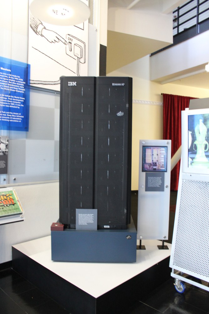
In 1997, IBM's (International Business Machines) Deep Blue computer beat the world chess champion. The success came mainly from search and from evaluation rules written by people, not from learning from data: Deep Blue belongs to classical artificial intelligence rather than to machine learning.
Deep learning, with networks of many layers trained on huge volumes of data, dominates image recognition and text processing today. Geoffrey Hinton, one of the authors of back-propagation, received the 2024 Nobel Prize in Physics for these contributions.
Conditions in finance are different. Price data are scarce compared with the millions of images in a training set, and the signal-to-noise ratio is low. Small networks are therefore the rule for financial forecasts, and the case study of Section 11 shows that even there extra layers add little.
where \(r_t\) is the return of day \(t\),\(x_{t-1}\) are the inputs known at the close of day \(t - 1\),\(f(x_{t-1})\) is the conditional mean, \(s^2(x_{t-1})\) is the conditional variance, and \(\varepsilon_t\) is a shock with mean 0 and variance 1. Both \(f\) and \(s^2\) are estimated by neural networks.
The ARCH (autoregressive conditional heteroskedasticity) model of Engle (1982) is a special case, with \(s^2(x) = \omega + \sum_i \alpha_i r_{t-i}^2\),\(\omega > 0\) and \(\alpha_i \ge 0\): the variance is a linear function of past squared returns. The network drops this form and lets the data determine how the variance depends on the past.
The NN-ARCH (neural-network ARCH) model thus keeps the mean-plus-volatility structure of Chapter 9 and makes only the shape of the functions flexible. The question is whether this flexibility adds anything to ARCH and GARCH.
In brief
Franke, Härdle & Hafner (2019), Ch. 19: \(r_t = f(x_{t-1}) + s(x_{t-1})\,\varepsilon_t\), with \(f\) and \(s^2\) estimated by neural networks
\(r_t\): the return of day \(t\); \(x_{t-1}\): the inputs known at the close of day \(t - 1\)
\(f(x_{t-1})\): the conditional mean; \(s^2(x_{t-1})\): the conditional variance; \(\varepsilon_t\): a shock with mean 0 and variance 1
ARCH (Engle (1982)) is the special case \(s^2(x) = \omega + \sum_i \alpha_i r_{t-i}^2\)
\(\omega > 0\), \(\alpha_i \ge 0\): the variance is a linear function of the past squared returns
The textbook's SFEnnarch Quantlet applies the model to GBP/USD. The inputs \(x\) are the last 3 returns of the exchange rate, the return on 10-year German bonds and the return on gold. Estimation has two steps: a network \(\hat f\) for the mean, with residuals \(e_t = r_t - \hat f(x_{t-1})\), then a network for \(e_t^2\), which gives the conditional variance \(\hat s^2(x_{t-1})\).
The network used, as in the Quantlet, is an RBF (radial basis function) network with 3 units. Unit \(j\) computes \(\exp(-\|x - c_j\|^2/s_j^2)\), where \(c_j\) is its centre, obtained by clustering, \(s_j\) is its width, and \(\|x - c_j\|\) is the distance from \(x\) to the centre. The unit is close to 1 when \(x\) is near \(c_j\) and close to 0 far from it; the network's output is a linear combination of the 3 units.
A technical problem arises in the second step: nothing in the network's construction forces \(\hat s^2 > 0\). A network for the variance needs a floor imposed from outside, while GARCH guarantees positivity through the restrictions on its parameters.
In brief
The Quantlet SFEnnarch: GBP/USD, inputs \(x\) = the last 3 returns, the German 10-year yield, the gold return
step 1: a network \(\hat f\) for the mean; residuals \(e_t = r_t - \hat f(x_{t-1})\)
step 2: a network for \(e_t^2\) gives the conditional variance \(\hat s^2(x_{t-1})\)
RBF (radial basis function) network with 3 units, as in the Quantlet
unit \(j\): \(\exp(-\|x - c_j\|^2/s_j^2)\); \(c_j\): its centre (found by clustering); \(s_j\): its width; \(\|x - c_j\|\): the distance from \(x\) to \(c_j\)
the unit is close to 1 when \(x\) is near \(c_j\) and close to 0 far from it; output: a linear combination of the 3 units
nothing forces \(\hat s^2 > 0\): a variance network needs a floor, which GARCH guarantees by its constraints
Question for the room With 5 RBF units instead of 3 (extra run), does the correlation of the network volatility with GARCH (0.45 with 3 units) rise or fall?
Answer
It rises to 0.61, and the maximum of the network goes from 22.0% to 27.6%; with 2 units the correlation falls to 0.26. More units give a more flexible shape, but the network still sees only the last 3 returns: the GARCH peak after the Brexit vote, 37.3%, stays far away.
The chart uses daily data from 7 January 2010, 4,048 days in all, and compares the annualised volatility given by the RBF network with that of a GARCH(1,1) estimated on the same data, with \(\hat\alpha = 0.077\) and \(\hat\beta = 0.892\).
On average, the two models agree: the mean volatility is 8.9% for the network and 8.8% for GARCH. Their paths differ, however: the correlation between them is only 0.45, and a small MLP estimated instead of the RBF network gives a similar correlation, 0.43.
The modest correlation shows that the two models do not say the same thing about when volatility is high. The next slide explains the difference through a specific episode.
In brief
Daily data from 7 January 2010 (4 048 days); annualised volatility of the RBF network and of GARCH(1,1) (\(\hat\alpha = 0.077\), \(\hat\beta = 0.892\))
Average volatility: network 8.9%, GARCH 8.8%; correlation of the two paths \(0.45\) (a small MLP: \(0.43\))
After the Brexit vote, the GARCH volatility peaks at 37.3% on 28 June 2016, while the network's reaches only 22.0%. The network sees only the last 3 returns: a large return raises its variance for 3 days, then the effect disappears. In the GARCH(1,1) model of Chapter 9,
the term \(\beta\,\sigma_{t-1}^2\), with \(\sigma_{t-1}^2\) yesterday's conditional variance, carries the whole past with geometrically declining weights. Volatility clustering needs memory, not only flexibility.
The network for the mean explains 0.08% of the variation of returns in sample: exchange rates are almost a random walk, and the useful part of the NN-ARCH model is the variance, as with GARCH.
The lesson goes beyond this example. Good features, such as the HAR averages of Section 7, which summarise the past over several horizons, matter more than the type of network. A flexible network with poor inputs cannot reconstruct information it does not receive.
In brief
After the Brexit vote, GARCH peaks at 37.3% (28 June 2016); the network only at 22.0%
the network sees only the last 3 returns: one large return raises its variance for 3 days, then the effect is gone
The textbook's SFEnnjpyusd Quantlet forecasts the yen–dollar rate from its last 3 values, with an RBF network with 3 units. The first 80% of the days are used for training, the last 20% for testing. The application in the chapter uses USD/JPY from 2000, with the split on 21 June 2021.
Forecasting the level has two pitfalls. First, a level series looks predictable because \(P_t \approx P_{t-1}\), and any model that follows yesterday's value has a small error in absolute terms. The right benchmark is therefore the random walk \(\hat P_t = P_{t-1}\) of Chapter 7. Second, a network with bounded units cannot extrapolate. Test levels climb to 163.9 yen, while the training maximum was 134.9.
The original code rescales the test forecasts using the range of the test series, which is not known in real time: a case of look-ahead bias. The chapter's version uses the training range, the only one available at the time of the forecast.
In brief
The Quantlet SFEnnjpyusd forecasts the yen–dollar rate from its last 3 values with an RBF network of 3 units
first 80% of the days for training, last 20% for testing; here USD/JPY from 2000, split on 21 June 2021
Two traps of level forecasting
a level series looks predictable because \(P_t \approx P_{t-1}\): the right benchmark is the random walk \(\hat P_t = P_{t-1}\) (Chapter 7)
a network with bounded units cannot extrapolate: the test levels go up to 163.9, the training maximum was 134.9
The original code rescales the test forecasts with the range of the test series, which is unknown in real time; here the training range is used
Question for the room With 90% of the days for training (extra run), how many times larger is the test RMSE of the network than that of the random walk?
Answer
13 times (12.12 against 0.91 yen), against 31 times with 80%. The training maximum rises to 151.6, but the test reaches 163.9: the network still cannot extrapolate beyond the levels it has seen.
The comparison uses the RMSE (root mean squared error), expressed in yen. On the training sample, the network has an RMSE of 2.64 and the random walk 0.66. On the test sample, the network has 27.56 and the random walk 0.89.
Out of sample, the network is 31 times worse than the rule "tomorrow = today". The huge difference comes from the second pitfall of the previous slide: when the rate leaves the training range, the RBF units approach zero and the forecast stays stuck below the observed levels.
The problem does not go away if the network forecasts returns instead of levels. On returns, the same network has an out-of-sample \(R^2\) of −0.14%: there is no signal to learn, and a zero forecast is better.
In brief
RMSE (root mean squared error) in yen: training: network 2.64, random walk 0.66; test: network 27.56, random walk 0.89
Interpretation: out of sample the network is 31 times worse than “tomorrow = today”; on returns the same network has an out-of-sample \(R^2\) of \(-0.14\%\)
An MLP, (13.4), is a linear regression in nonlinear features learned from the data and is trained by gradient descent and back-propagation. The textbook's NN-ARCH model gives an average volatility close to GARCH but, without long memory, reacts weakly to shocks such as the Brexit vote. On the USD/JPY level, a network is 31 times worse than the random walk. The next section applies all the models in a rigorous comparison for volatility.
Application: Forecasting Realised Volatility
The first application compares the chapter's models on the target most favourable to them: next week's volatility. The section defines the target and the features, the HAR benchmark and three evaluation tools, out-of-sample \(R^2\), QLIKE and the Diebold–Mariano test, then presents the results for the S&P 500 and Bitcoin, the forecasts in two crisis episodes and the importance of the features.
Here \(o_t\) is the overnight log return, from the previous close to the open, and \(u_t\),\(d_t\),\(c_t\) are the logs of the high, low and close relative to the open. The last two terms form the Garman & Klass (1980) estimator, which uses the day's range to reduce noise relative to the squared return.
The target is \(y_t = \ln\big(\tfrac15\sum_{j=1}^{5} v_{t+j}\big)\), the log of realised variance over the next week, that is over the next five trading days. It is known only at the close of day \(t + 5\), which makes the targets of neighbouring days overlap and calls for the purging of Section 3. The log brings the distribution of the target closer to the Normal distribution and guarantees positive forecasts after applying the exponential function.
In brief
Daily variance proxy of Chapter 8 (no intraday data): an estimate of the variance of day \(t\) from its open, high, low and close
The features are computed at the close of day \(t\). The HAR set contains three features: \(\ln v_t\), the log of the 5-day average of \(v\) (the week) and the log of the 22-day average (the month). The extended set has 11 features: in addition, 4 lags of \(\ln v_t\), from \(\ln v_{t-1}\) to \(\ln v_{t-4}\), the 66-day average, the return \(r_t\), its negative part \(\min(r_t, 0)\) and its absolute value \(|r_t|\).
The feature \(\min(r_t, 0)\) equals the return if it is negative and 0 otherwise. It lets falls and rises have different effects on future volatility, that is, the leverage effect. A linear model with \(r_t\) and \(\min(r_t, 0)\) has one slope for up days and another for down days.
The extended set gives flexible models the chance to find information beyond HAR: individual lags, a longer horizon and asymmetry. If a model beats HAR, these features and the nonlinearities between them are the possible sources of the gain.
In brief
Features at the close of day \(t\)
HAR: \(\ln v_t\), \(\ln\) of the mean over 5 days (week) and over 22 days (month)
extended (11): plus 4 lags of \(\ln v_t\) (\(\ln v_{t-1}, \dots, \ln v_{t-4}\)), the 66-day mean, \(r_t\), \(\min(r_t, 0)\), \(|r_t|\)
Notation
\(r_t\): the log return of day \(t\); \(|r_t|\): its absolute value
\(\min(r_t, 0)\): the return if negative, 0 otherwise; it lets falls and rises act differently (the leverage effect)
where \(v_t^{(w)}\) and \(v_t^{(m)}\) are the averages of \(v\) over the last 5 days and the last 22 days, \(\beta_0\) is the constant, \(\beta_d\),\(\beta_w\),\(\beta_m\) are the weights of the three horizons, and \(u_t\) is the error. The model is estimated by OLS.
The three components correspond to market participants with different horizons: daily, weekly and monthly. With positive weights on all three, a volatility shock stays in the monthly average long after it has left the daily one, so it decays slowly.
This slow decay mimics the long memory of volatility of Chapter 11, without the fractional parameters of a FIGARCH model. A linear model with four coefficients that reproduces this stylised fact is a hard benchmark to beat.
In brief
HAR (heterogeneous autoregressive) model Corsi (2009)
The question of the section is whether the lasso, a random forest, gradient boosting or an MLP add anything over HAR out of sample. On intraday data, the large study of Christensen, Siggaard & Veliyev (2023) finds modest gains, coming mostly from the extra features.
The evaluation uses the walk-forward scheme of Section 3, with yearly re-estimation: for the S&P 500 the forecasts start in 2013, for Bitcoin in 2018. All models receive the same data and the same rules for choosing hyperparameters.
The models forecast the log of variance, \(\hat y_t\), but evaluation by QLIKE requires a forecast of variance in levels. The transformation is \(\hat h_t = \exp(\hat y_t + \hat s^2/2)\), where \(\hat s^2\) is the residual variance in training. If the error in logs is approximately Normal, the variance has a log-Normal distribution and its mean is \(\exp(\hat y_t + \hat s^2/2)\);\(\exp(\hat y_t)\) alone would understate the mean variance.
In brief
The question of this section
do lasso, random forest, gradient boosting or an MLP add anything to HAR out of sample?
The out-of-sample \(R^2\), proposed by Campbell & Thompson (2008), compares the squared error of the model with that of a benchmark forecast \(\tilde y_t\):
where \(\hat y_t\) is the model's forecast and the sums run over the test days only. In the chapter, the benchmark \(\tilde y_t\) is either the training mean or the HAR forecast.
The measure is at most 1. A positive value means a smaller squared error than the benchmark's, a negative one a larger error. Unlike the in-sample \(R^2\),\(R^2_{OOS}\) can be negative, and negative values are common when flexible models are applied to noisy targets.
For the S&P 500, the squared error of the MLP is 0.397 and that of HAR is 0.433. The ratio is 0.917, so \(R^2_{OOS} = 1 - 0.917 = +8.3\%\): the MLP reduces the squared error of the HAR forecasts by 8.3%.
where \(\mathrm{RV}_t\) is the realised variance over the next 5 days, the target in levels, and \(\hat h_t\) is its forecast. Patton (2011) shows that QLIKE is robust to using a noisy proxy instead of the true variance: the ranking of models is not distorted by the noise of the proxy.
For a given \(\mathrm{RV}_t\), the loss is smallest at \(\hat h_t = \mathrm{RV}_t\), and a smaller average QLIKE indicates better forecasts. The loss is asymmetric, however. For \(\mathrm{RV} = 1\), the forecast \(\hat h = 0.5\) costs 1.307 and the forecast \(\hat h = 2\) costs 1.193, although both are off by a factor of 2.
Underestimation is therefore penalised more than overestimation. The asymmetry matches the costs in risk management, where underestimated volatility leads to insufficient capital and VaR violations, that is, to the more costly error.
The Diebold & Mariano (1995) (DM) test asks whether two models \(A\) and \(B\) have the same expected loss. Starting from the difference of the losses on each day,
where \(\bar d\) is the mean of \(d_t\) and \(n\) is the number of test days. Under the hypothesis of equal accuracy, the DM statistic is approximately standard Normal.
The denominator uses the long-run variance \(\widehat{\mathrm{LRV}}\) of \(d_t\), estimated by Newey–West with 5 lags. The correction is needed because the overlapping 5-day targets make the loss differences autocorrelated; the plain variance would understate the uncertainty of \(\bar d\) and make the test too lenient.
The sign of the statistic gives the direction: a negative DM means that model \(A\) has the smaller loss, a positive DM that \(B\) is better. If \(|\mathrm{DM}| > 1.96\), the difference is significant at the 5% level. In the following table, \(A\) is each machine learning model and \(B\) is HAR.
In brief
Diebold–Mariano test Diebold & Mariano (1995): do two models \(A\) and \(B\) have the same expected loss?
The table summarises the forecasts for 3,444 days of the S&P 500, from 2 January 2013, and for 3,178 days of Bitcoin, from 1 January 2018. \(R^2_{OOS}\) is expressed in percent and computed on the log of variance, relative to the training mean and relative to HAR; GB stands for gradient boosting.
For the S&P 500, HAR already has an \(R^2_{OOS}\) of 61.5% relative to the mean. The lasso and the MLP beat it significantly: \(R^2_{OOS}\) relative to HAR is +7.1% for the lasso and +8.3% for the MLP, with DM statistics of −5.12 and −3.96, both with p-values below 0.001, and QLIKE falls from 0.414 to 0.400 and 0.398. The random forest (+1.0%, p 0.747) and boosting (−2.7%, p 0.308) do not differ significantly from HAR.
For Bitcoin, HAR has an \(R^2_{OOS}\) of 44.0% relative to the mean, and no model beats it significantly: the lasso gains +2.0%, but with a p-value of 0.520. Boosting is significantly worse than HAR, with \(R^2_{OOS}\) of −4.2% and DM +2.12 (p 0.034). The gains, where they exist, are a few percent, and they come from the models closest to HAR: the lasso is an extended, penalised HAR, and the MLP uses the same inputs.
In brief
Model
\(R^2_{OOS}\) vs. mean
\(R^2_{OOS}\) vs. HAR
QLIKE
DM vs. HAR (p)
S&P 500
HAR
\(61.5\)
–
\(0.414\)
–
Lasso
\(64.2\)
\({+7.1}\)
\(0.400\)
\({-5.12}\) (\(<\) 0.001)
RF
\(61.9\)
\({+1.0}\)
\(0.416\)
\({+0.32}\) (0.747)
GB
\(60.4\)
\({-2.7}\)
\(0.421\)
\({+1.02}\) (0.308)
MLP
\(64.7\)
\({+8.3}\)
\(0.398\)
\({-3.96}\) (\(<\) 0.001)
Bitcoin
HAR
\(44.0\)
–
\(3.111\)
–
Lasso
\(45.1\)
\({+2.0}\)
\(3.108\)
\({-0.64}\) (0.520)
RF
\(43.4\)
\({-1.2}\)
\(3.119\)
\({+0.81}\) (0.418)
GB
\(41.7\)
\({-4.2}\)
\(3.148\)
\({+2.12}\) (0.034)
MLP
\(43.8\)
\({-0.3}\)
\(3.123\)
\({+1.10}\) (0.272)
Forecasts for 3 444 days (S&P 500, from 2 January 2013) and 3 178 days (Bitcoin, from 1 January 2018); \(R^2_{OOS}\) in %, on log RV; GB: gradient boosting
S&P 500: lasso and MLP beat HAR significantly (\(+7.1\%\), \(+8.3\%\)); random forest and boosting do not
Bitcoin: no model beats HAR; boosting is significantly worse (DM \(+2.12\))
Question for the room Fold 2020, the day with the highest HAR forecast (18 March 2020): is the forecast above or below the volatility realised over the next 5 days?
Answer
Slightly above: 69.3% against 66.1% per year. The peak of the realised volatility in 2020, 102.4%, came before the peak of the forecast: HAR reacts after the shock, it does not anticipate it.
Question for the room ▶ moves to the random forest (S&P 500, against HAR). What is R²_OOS?
Answer
+1.0%: MSE 0.429 against 0.433. Against the training mean the same model has 61.9%: R²_OOS depends on the benchmark, and HAR is a much tougher one. The DM test does not separate this gain from noise (p = 0.747).
Question for the room RV = 1: which forecast costs more in QLIKE, ĥ = 1/3 or ĥ = 3?
Answer
ĥ = 1/3: 3 + ln(1/3) = 1.901, against 1/3 + ln 3 = 1.432. Underestimating three times costs more than overestimating three times, although the squared error ranks them the other way: (1 − 1/3)² = 0.444 and (1 − 3)² = 4.
Question for the room ▶ lowers the number of Newey–West lags from 5 to 0. What happens to the DM statistic of the MLP against HAR (S&P 500, −3.96)?
Answer
It grows in absolute value, to −4.61: the long-run variance with 5 lags is 1.35 times the plain variance, because the 5-day targets overlap and make d_t autocorrelated. Without the correction the test looks surer than it is; here the conclusion (MLP better) stays the same.
Out-of-sample results: R²_OOS on log RV (%), QLIKE, DM statistic against HAR (p-value)
Question for the room ▶ moves to the test days from 2020. Is the MLP still significantly better than HAR on the S&P 500 at 5%?
Answer
Yes: R²_OOS +7.9%, DM −2.28 (p = 0.023); lasso +7.4%, DM −3.42. The random forest and boosting are not significantly better than HAR in either subperiod: up to 2019 they have −1.5% and −11.0%, from 2020 +3.5% and +5.8%, with p above 0.6.
Question for the room In 2020, is the peak of the random-forest forecast above or below the peak of the realised volatility (102% per year)?
Answer
Far below: 53%, against 69% for HAR and 159% for the MLP. A random forest predicts averages of training leaves, so it stays below extreme values; the MLP and the lasso (172%) extrapolate and can overshoot the target.
The chart shows, for the S&P 500, the annualised realised volatility over the next 5 days, \(\sqrt{252\,\mathrm{RV}_t}\), and the HAR, random forest and MLP forecasts made at the close of day \(t\), in two crisis episodes: March 2020 and April 2025.
All models react only after the first shock. No feature built from past volatility can announce a jump in volatility before it starts; the models adjust quickly after the first turbulent day, but cannot anticipate it.
After the shock, the models differ in how they extrapolate. The random forest is capped by the largest values seen in training, because its forecast is an average of leaves that contain historical observations. The MLP has no such cap and can overshoot the target on the most turbulent days.
In brief
S&P 500: annualised realised volatility of the next 5 days, \(\sqrt{252\,\mathrm{RV}_t}\), and the HAR, random forest and MLP forecasts made at the close of day \(t\)
Interpretation: all models react only after the first shock (March 2020, April 2025); the forest is capped by the largest values it saw in training, the MLP can overshoot
Permutation importance shuffles the values of one feature in the test data and measures how much the test MSE rises. A large rise shows that the model relies on that feature. Correlated features share their importance, however: if one is shuffled, the model can use another similar one, so each looks less important than the group.
Shapley values, from game theory, decompose each forecast: \(\hat f(x) = \phi_0 + \sum_j \phi_j(x)\). Here \(\phi_0\) is the average forecast, and \(\phi_j(x)\) is the contribution of feature \(j\) to this forecast: positive if the feature raises the forecast above the average, negative if it lowers it. The contribution \(\phi_j\) is the average change in \(\hat f\) when \(j\) is added to each subset of the other features. SHAP (Shapley additive explanations), by Lundberg & Lee (2017), offers fast versions for trees; for a linear model, \(\phi_j = \beta_j(x_j - \bar x_j)\).
Both tools describe the model, not the economy. An important feature is one the model uses for forecasting, which does not mean that it causes future volatility.
In brief
Permutation importance: shuffle one feature in the test data and measure how much the test MSE rises
large increase: the model relies on the feature; correlated features share (and hide) their importance
Shapley values (game theory): \(\hat f(x) = \phi_0 + \sum_j \phi_j(x)\), \(\phi_j\) the fair share of feature \(j\) in the forecast
\(\phi_0\): the average forecast; \(\phi_j(x) > 0\): feature \(j\) raises this forecast above the average, \(\phi_j(x) < 0\): lowers it
\(\phi_j\) averages the change of \(\hat f\) when \(j\) joins every subset of the other features
SHAP (Shapley additive explanations) Lundberg & Lee (2017): fast versions for trees; for a linear model \(\phi_j = \beta_j(x_j - \bar x_j)\)
Both describe the model, not the economy: importance is not causality
Permutation importance (10 shuffles) and mean |φ| (random forest on the 3 HAR features)
Question for the room ▶ shows log RV day only. Is the range of its Shapley values wider or narrower than for log RV week?
Answer
Narrower: daily φ between −0.32 and 0.35, against −0.66 and 2.25 for the week; mean |φ| 0.13 against 0.52. The forest relies on the weekly variance, which already contains part of the information of the day.
The left panel shows permutation importance for a random forest on the 11 features, trained up to 2019 and tested in 2020–2026, on 1,682 days. Shuffling the weekly variance raises test MSE by 0.201, the monthly variance by 0.053 and the daily variance by 0.034. The other features matter much less.
The right panel uses the exact Shapley values of a random forest on the 3 HAR features. The mean of \(|\phi|\) is 0.52 for the weekly component, 0.13 for the monthly and 0.13 for the daily one. The effect of the weekly component is nonlinear and grows with the level of volatility.
The two methods and three models of the chapter, the lasso, the depth-2 tree and the random forest, reach the same conclusion: the weekly variance is the main feature. The random forest adds a nonlinear shape to this dependence, but not a new source of information.
In brief
Left: random forest on 11 features, trained to 2019, tested 2020–2026 (1 682 days): shuffling the weekly variance raises the MSE by \(0.201\), the monthly by \(0.053\), the daily by \(0.034\)
Right: exact Shapley values of a forest on the 3 HAR features; mean \(|\phi|\): week \(0.52\), month \(0.13\), day \(0.13\); the effect is nonlinear and grows with the level of volatility
HAR, (13.5), is a strong benchmark for volatility. Evaluated by \(R^2_{OOS}\),(13.6), QLIKE, (13.7), and the Diebold–Mariano test, (13.8), on the S&P 500 the lasso and the MLP beat it significantly by 7.1% and 8.3%, while the random forest and boosting do not; on Bitcoin no model beats it. All models react only after the first shock of a crisis, and the weekly variance dominates feature importance. The next section applies the same methods to a target with much less signal, the sign of the return.
Application: the Sign of Tomorrow's Return
The second application is a classification problem: forecasting the direction of tomorrow's return. The section defines the target and the models, sets the right benchmark, the majority class, and a test against it, then compares the accuracy of the models for the S&P 500, the BET and Bitcoin.
The target is \(y_t = \mathbf{1}\{r_{t+1} > 0\}\), where \(\mathbf{1}\{\cdot\}\) is the indicator function, equal to 1 if the statement is true and 0 otherwise; \(y_t = 1\) means that tomorrow's return is positive. The features, computed at the close of day \(t\), are the last 5 returns, the sums of returns over 5, 21 and 63 days and the volatility over 21 and 63 days.
The models are the logit regression of Chapter 12 and random forest and gradient boosting classifiers, estimated with the walk-forward scheme and yearly re-estimation. The data are the S&P 500 and the BET (Bucharest Exchange Trading), the benchmark index of the Bucharest Stock Exchange (BVB), from 2008, and Bitcoin from 2018. The measures, defined in Chapter 12, are accuracy, the share of days with the sign forecast correctly, and the AUC (area under the ROC curve), the area under the ROC (receiver operating characteristic) curve, for which 0.5 means no ranking ability.
Expectations are modest for theoretical reasons. Weak-form efficiency, from Chapter 7, says that any reliable pattern in past returns would be exploited by trading and would disappear. A model that nevertheless finds such a pattern must be checked all the more carefully.
In brief
Target: \(y_t = \mathbf{1}\{r_{t+1} > 0\}\); features at the close of day \(t\): the last 5 returns, sums over 5, 21 and 63 days, volatility over 21 and 63 days
\(\mathbf{1}\{\cdot\}\): the indicator, 1 if the condition holds and 0 otherwise; \(y_t = 1\): tomorrow's return is positive
models: logit (Chapter 12), random forest and gradient boosting classifiers; walk-forward, yearly refits
The benchmark for classification is the majority class: always forecast the more frequent class in the training sample, here "up". For the S&P 500 since 2008, 54.4% of days are up days, so the rule "always up" is right on 54.4% of days. An accuracy of 53% looks like skill, being above 50%, but against this benchmark it is a loss.
The difference from the benchmark is tested with the statistic
where \(\widehat{\mathrm{acc}}\) is the model's accuracy, \(\mathrm{acc}_0\) the benchmark's accuracy and \(n\) the number of test days. If the model has no real edge, \(z\) is approximately standard Normal. For the S&P 500, with \(n = 4{,}705\), the standard error is 0.73 percentage points, so the 95% band around the benchmark has a width of ±1.4 points.
The random forest has an accuracy of 53.1%, with \(z = -1.79\) (p 0.074), and boosting 52.1%, with \(z = -3.19\) (p 0.001): boosting is significantly worse than the rule "always up". For forecasts of the returns themselves, the corresponding benchmark is the zero forecast or the historical mean (Welch & Goyal, 2008).
In brief
Majority-class baseline: always forecast the more frequent class of the training sample (here: “up”)
S&P 500 since 2008: 54.4% of the days are up, so “always up” is right on 54.4% of the days
an accuracy of 53% sounds like skill; against this baseline it is a loss
Test against the baseline: \(z = (\widehat{\mathrm{acc}} - \mathrm{acc}_0)/\sqrt{\mathrm{acc}_0(1 - \mathrm{acc}_0)/n}\)
\(\widehat{\mathrm{acc}}\): the accuracy of the model; \(\mathrm{acc}_0\): that of the baseline; \(n\): the test days; \(z \approx N(0,1)\) if the model has no extra skill
S&P 500, \(n = 4\,705\): standard error 0.73 points; a 95% band of \(\pm\)1.4 points around the baseline
Question for the room BET instead of the S&P 500, random forest: what is the z statistic against the baseline?
Answer
−0.21 (53.6% against 53.8%, p = 0.84). On the S&P 500 the random forest has z = −1.79, on Bitcoin −0.99: on no market is a model significantly better than “always up”.
Question for the room ▶ tests only up to 2012 (5 years). Is any model significantly worse than the baseline on the S&P 500?
Answer
Yes: gradient boosting, −3.9 points, z = −2.77; logit and the random forest have z = −1.36 and −1.30. The 95% band is wider with fewer days, yet boosting stays outside it: the model learns patterns from the noise of the training years.
The chart shows, for each market and each model, accuracy minus the benchmark's accuracy, in percentage points. The grey band covers ±1.96 standard errors around zero: a model inside the band does not differ significantly from the rule "always up".
The AUC confirms the picture. For the logit and the random forest, the AUC is 0.511 and 0.507 on the S&P 500, 0.533 and 0.533 on the BET, 0.515 and 0.519 on Bitcoin. All values are very close to 0.5, that is, the models hardly rank the days by their probability of an up move.
The logit forecasts "up" on 86% of S&P 500 days. Its estimated probabilities are almost constant, slightly above 0.5, so the logit behaves almost like the benchmark. This explains why it loses little against the benchmark, while the flexible models lose more.
In brief
Accuracy minus the baseline accuracy (percentage points); band: \(\pm 1.96\) standard errors around zero
AUC of the logit and of the forest: S&P 500 0.511 and 0.507, BET 0.533 and 0.533, Bitcoin 0.515 and 0.519; logit forecasts “up” on 86% of S&P 500 days
On no market is any model significantly better than the rule "always up", and the flexible models are worse than the logit. On the S&P 500, the differences from the benchmark are −0.6 points for the logit, −1.3 for the random forest and −2.3 for boosting; on Bitcoin, +0.1 for the logit and −0.9 for the random forest.
The explanation is the very low signal-to-noise ratio of daily returns. In terms of the decomposition (13.1), almost all of the error is noise. The flexible models find patterns in the noise of the training years, as in Section 2, and apply them to years in which the patterns no longer exist; the logit stays close to the benchmark precisely because it barely moves.
Even a real edge of one percentage point would rarely remain profitable: a daily strategy based on the sign trades very often, and transaction costs would eat the gain. The documented gains of machine learning in return forecasting come from large cross-sections at monthly horizons, not from a single index for the next day, as the case study of Section 11 shows.
In brief
No model beats “always up” significantly on any market; the flexible models do worse than the logit
The signal-to-noise ratio of daily returns is tiny
flexible models find patterns in the noise of the training years (Section 2); the logit is close to the baseline because it hardly moves
Even a real edge of one point would rarely survive costs: a daily sign strategy trades very often
ML gains in returns come from large cross-sections at monthly horizons, not from one index tomorrow (Section 11)
Section summary
The forecast of the sign of tomorrow's return is judged against the majority-class rule, which for the S&P 500 is right on 54.4% of days. No model, on any market, is significantly better than this rule; the AUC stays close to 0.5, and the flexible models are worse than the logit. The next section returns to risk, with the forecast of a quantile.
Application: VaR 1% by Quantile Methods
The third application forecasts VaR 1% directly as a conditional quantile. The section introduces quantile regression and the quantile loss, its version with boosted trees, and compares them by backtesting with historical simulation and with GARCH-t on the S&P 500 and Bitcoin.
The quantile regression of Koenker & Bassett (1978) estimates the conditional quantile of order \(\alpha\),\(q_\alpha(x) = x^\top\beta_\alpha\). The quantile \(q_\alpha(x)\) is the level below which \(y\) lies with probability \(\alpha\), conditional on \(x\), and the coefficients \(\beta_\alpha\) are specific to the level \(\alpha\): the same feature can have different effects on the tail and on the centre of the distribution.
Estimation minimises the quantile loss. For an error \(u = y - q\),
An observation below the quantile (\(u < 0\)) costs \((1 - \alpha)|u|\), and one above it costs \(\alpha|u|\). For \(\alpha = 0.5\) the two costs are equal and we obtain median regression.
With \(\alpha = 0.01\), observations below the quantile are 99 times more expensive than those above it. The minimum of the average loss is reached when about 1% of the observations lie below \(q\), which is exactly the property that defines the 1% quantile.
In brief
Koenker & Bassett (1978): estimate the conditional \(\alpha\)-quantile \(q_\alpha(x) = x^\top\beta_\alpha\) by minimising the quantile (pinball) loss
\(q_\alpha(x)\): the level below which \(y\) falls with probability \(\alpha\), given \(x\); \(\beta_\alpha\): coefficients specific to the level \(\alpha\)
With \(\alpha = 0.01\) and \(q = -\mathrm{VaR}\), the loss (13.9) becomes the average quantile loss of Chapter 10: \((\alpha - I_t)(r_t + \mathrm{VaR}_t)\), where \(I_t = 1\) if \(r_t < -\mathrm{VaR}_t\), that is, if a violation occurs, and 0 otherwise. The same function thus serves both for estimating and for evaluating VaR forecasts.
VaR 1% for day \(t + 1\) is \(\widehat{\mathrm{VaR}}_t = -\hat q_{0.01}(x_t)\), with features \(x_t\): the daily, weekly and monthly volatility, computed as square roots of the proxy, and the return \(r_t\). No distribution of returns is assumed: the data choose how volatility translates into the 1% tail. CAViaR (Engle & Manganelli, 2004) is a dynamic version of this idea, in which yesterday's quantile enters the equation for today's quantile.
Quantile gradient boosting (QGB) uses the same loss, with trees added by boosting as in Section 5. It is more flexible than linear regression, but at the 1% level each leaf sees few observations from the tail, so the variance of the estimate is high.
In brief
With \(\alpha = 0.01\) and \(q = -\mathrm{VaR}\): the average quantile loss of Chapter 10
\((\alpha - I_t)(r_t + \mathrm{VaR}_t)\), with \(I_t = 1\) if \(r_t < -\mathrm{VaR}_t\) (an exception) and 0 otherwise
VaR 1% for day \(t + 1\): \(\widehat{\mathrm{VaR}}_t = -\hat q_{0.01}(x_t)\), with \(x_t\) = daily, weekly and monthly volatility (square roots of the proxy) and \(r_t\)
no distribution is assumed: the data choose how volatility maps into the tail; CAViaR Engle & Manganelli (2004) is a dynamic version
Quantile gradient boosting: the same loss with boosted trees (Section 5)
flexible, but at 1% each leaf sees few tail observations: high variance
Backtest of VaR 1%: Quantile Methods, HS and GARCH-t (1/2)
The table compares four methods. QR is linear quantile regression, and QGB is quantile gradient boosting. The benchmarks are 500-day historical simulation (HS) and a GARCH-t re-estimated every January, both from Chapter 10.
Column \(x\) gives the number of violations, the days with \(r_{t+1} < -\widehat{\mathrm{VaR}}_t\), among the \(n\) test days, and the rate is \(x/n\), with target 1%. "Kupiec p" is the p-value of the Kupiec (1995) test of the violation rate, and "ind. p" is the p-value of the Christoffersen (1998) independence test. The average quantile loss, multiplied by 100, measures the quality of the forecasts as a whole (lower is better), and "mean VaR" is the average VaR 1%, in percent.
On the S&P 500, QR has 28 violations, a rate of 0.81% and the smallest loss, 3.38; GARCH-t has 52 violations, a rate of 1.51% and a Kupiec p of 0.005. On Bitcoin, HS has 32 violations, a rate of 1.01%, and QGB has 47 violations, with a rate of 1.48%. Mean VaR ranges from 2.42% (GARCH-t) to 2.97% (HS) for the S&P 500 and from 8.52% (GARCH-t) to 10.46% (QR) for Bitcoin.
In brief
Method
\(x\)
rate (%)
p Kupiec
p ind.
loss \(\times 100\)
mean VaR
S&P 500
QR
28
\(0.81\)
0.252
0.020
\(3.38\)
\(2.70\)
QGB
42
\(1.22\)
0.213
0.015
\(3.51\)
\(2.46\)
HS
46
\(1.33\)
0.061
\(<\) 0.001
\(4.78\)
\(2.97\)
GARCH-t
52
\(1.51\)
0.005
0.008
\(3.50\)
\(2.42\)
Bitcoin
QR
23
\(0.72\)
0.098
0.563
\(13.03\)
\(10.46\)
QGB
47
\(1.48\)
0.012
0.235
\(13.19\)
\(8.86\)
HS
32
\(1.01\)
0.974
0.332
\(13.01\)
\(9.30\)
GARCH-t
41
\(1.29\)
0.117
0.558
\(13.15\)
\(8.52\)
Columns
\(x\): the number of exceptions (\(r_{t+1} < -\widehat{\mathrm{VaR}}_t\)) in \(n\) test days; rate \(= x/n\), target 1%
p Kupiec: p-value of the Kupiec test of the rate; p ind.: p-value of the Christoffersen test of independence (Chapter 10)
loss \(\times 100\): the mean quantile loss (smaller is better); mean VaR: the average VaR 1%, in %
Methods
QR: linear quantile regression; QGB: quantile gradient boosting
HS: historical simulation on 500 days; GARCH-t: re-estimated each January (Chapter 10)
On the S&P 500, with 3,448 test days from 2 January 2013, quantile regression has a violation rate consistent with 1% (0.81%) and the smallest quantile loss. Its violations are not fully independent: the p-value of the independence test is 0.020. GARCH-t is violated too often, on 1.51% of days, and the Kupiec test rejects it.
On Bitcoin, with 3,182 test days, historical simulation has the best rate, 1.01%. Quantile gradient boosting is rejected by the Kupiec test, with a rate of 1.48% and a p-value of 0.012: its flexibility does not make up for the small number of observations in the tail.
Reading the p-values follows Chapter 10. A Kupiec p below 0.05 shows that the violation rate differs significantly from 1%. An ind. p below 0.05 shows that violations come in clusters, that is, VaR reacts too slowly to rises in volatility and lets several violations through on consecutive days.
In brief
S&P 500 (3 448 days from 2 January 2013): QR has the right rate (0.81%) and the smallest loss
its exceptions are not fully independent (p ind. 0.020)
GARCH-t is exceeded too often (1.51%)
Bitcoin (3 182 days): HS has the best rate (1.01%)
QGB is rejected by the Kupiec test (1.48%, p 0.012)
Reading the p-values
p Kupiec below 0.05: the exception rate differs significantly from 1%
p ind. below 0.05: the exceptions come in clusters, so the VaR reacts too slowly
Worked example: the quantile loss on the S&P 500 returns
\[\rho_\alpha(u) = u\,(\alpha - \mathbf{1}\{u < 0\}), \qquad u = y - q, \qquad \hat q = \arg\min_q \frac1n\sum_t \rho_\alpha(y_t - q)\]
Question for the room With α = 0.05, which constant forecast q minimises the mean loss on the S&P 500 test returns?
Answer
q = −1.59%, the empirical 5% quantile: 4.99% of the days lie below it. For α = 0.01 the minimum is at −3.07% (0.99% of the days below). The mean return, 0.05%, minimises the squared error, not the quantile loss.
Backtest of VaR 1% (the table of the slide)
Question for the room ▶ moves to the test days from 2020. Does the Kupiec test reject the exceedance rate of GARCH-t on the S&P 500 at 5%?
Answer
Yes: 1.60% (27 of 1,686 days), p = 0.022. QR has 0.71% (p = 0.21), and the HS exceedances cluster (p ind. 0.005). For Bitcoin from 2020, QR is exceeded too rarely: 0.45%, p Kupiec 0.002.
Question for the room In 2025 (up to September), which method has the most exceedances on the S&P 500?
Answer
HS: 5 exceedances, against 4 for GARCH-t and 1 each for QR and QGB. After 500 calm days, historical simulation enters April 2025 with a VaR that is too small and reacts slowly.
The chart shows, for the S&P 500, the next-day returns and minus VaR 1% for the four methods, in 2020 and 2025; the dots mark the violations of the VaR obtained by quantile regression.
QR and GARCH-t follow volatility: when volatility rises, their threshold drops within a few days. HS reacts slowly, because the 500-day window changes only as new days enter, one at a time, and an extreme day moves the 1% quantile only after several such days have entered the window.
The difference shows in 2020: HS was violated 10 times and QR 4 times, and the HS violations come in clusters, which explains the independence-test p-value below 0.001 in the table. A method that follows current volatility avoids exactly these runs of violations.
In brief
S&P 500: next-day returns and minus VaR 1% of the four methods; dots: exceedances of the quantile-regression VaR
Interpretation: QR and GARCH-t move with volatility; HS reacts only slowly; in 2020 HS was exceeded 10 times, QR 4 times, and the HS exceptions cluster (p ind. \(<\) 0.001)
Quantile regression estimates VaR 1% directly, through the quantile loss (13.9), without assumptions on the distribution. On the S&P 500, the linear version has the right violation rate and the smallest loss, while GARCH-t is violated too often; on Bitcoin, historical simulation has the best rate, and quantile boosting is rejected, because at 1% it has too few tail observations. The next section treats a problem common to all model comparisons: the number of trials.
Data Snooping and the Deflated Sharpe Ratio
The section quantifies the optimism that arises when the best of many strategies tried on the same data is reported. It computes the expected maximum of the Sharpe ratios of strategies without skill, illustrates it with 30 moving-average rules on the S&P 500 and introduces the deflated Sharpe ratio, which corrects for the number of trials.
Data snooping means trying many models or rules on the same data and reporting the best (White, 2000). With enough trials, a rule without any skill looks excellent in sample, because the maximum of many noisy estimates lies systematically above their true value. Harvey, Liu & Zhu (2016) show that hundreds of published return predictors would not survive a correction for multiple testing.
The Sharpe ratio is the mean excess return divided by its standard deviation (Chapter 1). For a strategy without skill, the annual Sharpe ratio estimated on \(Y\) years of data is approximately \(N(0, 1/Y)\). The zero mean expresses the lack of skill, and the variance \(1/Y\) is the estimation error, which falls with the length of the sample.
Over 10 years, the standard deviation of the estimated Sharpe ratio is \(1/\sqrt{10} = 0.316\). A strategy without skill thus has a reasonable chance of showing a Sharpe ratio of 0.3 or more by luck alone, and when many strategies are tried, the best of them will look much better.
In brief
Data snooping: trying many models or rules on the same data and reporting the best White (2000)
with enough trials, a rule without skill looks excellent in sample
hundreds of published return predictors would not survive a multiple-testing correction Harvey, Liu & Zhu (2016)
The annual Sharpe ratio of a strategy without skill over \(Y\) years is about \(N(0, 1/Y)\)
Sharpe ratio: mean excess return divided by its standard deviation (Chapter 1); \(Y\): the number of years of data
mean 0: no skill; variance \(1/Y\): the estimation error, which falls with the length of the sample
where \(\sigma\) is the standard deviation of the Sharpe ratios across trials, \(1/\sqrt{Y}\) in the case above, \(N\) is the number of trials, \(\Phi^{-1}\) is the quantile function of the standard Normal distribution, \(e \approx 2.718\), and \(\gamma = 0.5772\) is the Euler–Mascheroni constant.
The term \(\Phi^{-1}(1 - 1/N)\) grows roughly like \(\sqrt{2\ln N}\). The advantage given by luck thus grows slowly with the number of trials, but without limit: ten times more trials always add something to the best apparent result.
For 10 years, with \(\sigma = 0.316\) and \(N = 100\), the formula gives \(0.316\,[(1 - \gamma)\,2.326 + \gamma\,2.680] = 0.80\). An annual Sharpe ratio of 0.80 therefore appears, on average, by luck alone if the best of 100 strategies is chosen. In a simulation, the best of 10, 100 and 1,000 strategies without skill has an average Sharpe ratio of 0.48, 0.79 and 1.02.
Question for the room With 20 years of data instead of 10, what is the expected maximum for N = 100?
Answer
0.566 = 0.800/√2, because σ = 1/√20 = 0.224; the simulation gives 0.559. More years reduce the selection bias only by √Y: with N = 1,000 the maximum is still 0.728.
Worked example: the deflated Sharpe ratio of the best MA rule
Question for the room Up to which number of rules tried does the best MA rule stay significant (DSR > 0.95)?
Answer
Up to N = 6: DSR = 0.961 at N = 5, 0.955 at N = 6 and 0.949 at N = 7; at N = 30, 0.884. Without the correction (PSR) the rule would look significant, with 0.994: SR₀ grows slowly with N, but SR̂ = 0.0416 per day has a thin margin.
Question for the room ▶ tries only the first 10 rules. Which is the best in sample, and what is its rank after 2014?
Answer
MA 5/200 (Sharpe 0.57 in sample), with 0.74 after 2014, rank 3 of 30. With all 30 rules the winner, MA 50/200 (0.66), ends at rank 22: choosing among more rules raises the in-sample Sharpe ratio, not the future one.
The left panel shows the best annual Sharpe ratio among \(N\) strategies without skill, over 10 years, as a function of \(N\): the curve rises slowly, as in (13.10). The right panel moves to real data: 30 moving-average (MA) rules on the S&P 500, each invested in the index or in cash according to its signal, evaluated in 2000–2014 and then in 2015–2026.
The best rule in sample, MA 50/200, has a Sharpe ratio of 0.66. In the following period, the same rule achieves 0.54, 22nd of 30, below the buy-and-hold strategy, which has 0.72.
The in-sample and out-of-sample Sharpe ratios have a correlation of 0.04: the ranking of the rules in the first period says practically nothing about their ranking in the second. Selecting the best rule mostly selected the luck of the first period.
In brief
Left: the best annual Sharpe ratio among \(N\) strategies without skill (10 years); right: 30 moving-average rules on the S&P 500 (long or cash), 2000–2014 against 2015–2026
Interpretation: the best rule in sample (MA 50/200, Sharpe \(0.66\)) earns \(0.54\) afterwards, rank 22 of 30, below buy and hold (\(0.72\)); in and out of sample Sharpe ratios correlate \(0.04\)
The deflated Sharpe ratio (DSR) of Bailey & López de Prado (2014) is the probability that the true Sharpe ratio exceeds what the best of \(N\) trials would show by luck:
Here \(\widehat{SR}\) is the daily Sharpe ratio of the chosen strategy, \(T\) is the number of days, and \(SR_0\) is the expected maximum from (13.10), computed with \(\sigma\) equal to the standard deviation of the \(N\) Sharpe ratios tried. \(\hat\gamma_3\) is the skewness and \(\hat\gamma_4\) the kurtosis of daily returns, with value 3 for the Normal distribution; \(\Phi\) is the standard Normal distribution function.
The DSR is a probability in the interval \((0, 1)\). A value above 0.95 indicates a Sharpe ratio that is significant after correcting for the \(N\) trials. The denominator measures the precision of the estimate \(\widehat{SR}\): negative skewness and heavy tails, common in financial strategies, enlarge it and reduce the DSR, because a Sharpe ratio estimated from such returns is less precise.
In brief
Bailey & López de Prado (2014): the probability that the true Sharpe ratio exceeds what the best of \(N\) trials would show by luck
\(\widehat{SR}\): the per-day Sharpe ratio of the chosen strategy; \(T\): the number of days
\(SR_0\): the expected maximum of \(N\) zero-skill trials (above), with \(\sigma\) = the standard deviation of the \(N\) Sharpe ratios tried
\(\hat\gamma_3\): the skewness, \(\hat\gamma_4\): the kurtosis of the daily returns (3 for the Normal distribution); \(\Phi\): the standard Normal distribution function
Reading
the DSR is a probability in \((0, 1)\); above 0.95: the Sharpe ratio is significant after the correction for \(N\) trials
negative skewness and fat tails enlarge the denominator and lower the DSR
The step-by-step calculation uses the best MA rule, with \(N = 30\) rules tried and \(T = 3{,}769\) days. The daily Sharpe ratio is \(\widehat{SR} = 0.0416\), that is \(0.0416 \times \sqrt{252} = 0.66\) per year; the skewness of daily returns is \(\hat\gamma_3 = -0.44\) and the kurtosis \(\hat\gamma_4 = 12.0\).
The luck threshold is \(SR_0 = 0.0105\,[(1 - \gamma)\,1.834 + \gamma\,2.249] = 0.0219\) per day, that is 0.35 per year. The argument of \(\Phi\) in (13.11) is \(z = 1.20\), so DSR \(= \Phi(1.20) = 0.88\). Without the correction for \(N\), with \(SR_0 = 0\), we obtain the probabilistic Sharpe ratio (PSR), equal to 0.994.
Taken alone, the rule looks significant: the PSR is well above 0.95. After correcting for the 30 trials, the DSR falls to 0.88, below the 0.95 threshold, and the Sharpe ratio is no longer significant. The result in 2015–2026, 22nd of 30, confirms this conclusion.
In brief
Step by step: the best MA rule, \(N = 30\), \(T = 3\,769\) days
\(\widehat{SR} = 0.0416\) per day (\(\times\sqrt{252} = 0.66\)); \(\hat\gamma_3 = -0.44\), \(\hat\gamma_4 = 12.0\)
\(z\), the argument of \(\Phi\) in the DSR formula: \(z = 1.20\), so DSR \(= \Phi(z) = 0.88\)
without the correction for \(N\) (PSR, probabilistic Sharpe ratio, \(SR_0 = 0\)): \(0.994\)
Interpretation: alone the rule looks significant; after 30 trials it is not (DSR below 0.95), as its later performance confirms
Section summary
The best of \(N\) strategies without skill has a positive Sharpe ratio that grows with \(N\),(13.10): over 10 years, about 0.80 for 100 trials. On the S&P 500, the best of 30 moving-average rules ends up 22nd in the following period, and the DSR, (13.11), shows that its Sharpe ratio is not significant after the correction. The number of trials must therefore be reported together with the result. The next section presents a paper in which machine learning passes these tests.
Case Study: Gu, Kelly and Xiu (2020)
The section presents the reference paper of the field, which compares machine learning methods for the monthly returns of US stocks. It describes the data and the estimation scheme, the evaluation, the statistical and economic results and their limits.
Gu, Kelly & Xiu (2020) ask which methods best predict the monthly return of individual US stocks. The data cover almost 30,000 stocks over 1957–2016. The features are 94 firm characteristics, interacted with 8 macroeconomic variables, plus 74 industry dummy variables: 920 features in all.
The estimation scheme is of the walk-forward type: 18 years of training (1957–1974), 12 years of validation (1975–1986) and 30 years of testing (1987–2016). The models are re-estimated once a year; the training window grows and the validation window moves forward, so that each forecast uses only earlier data.
The paper compares OLS, penalised and dimension-reduction regressions, random forests, boosted trees and neural networks with 1 to 5 hidden layers, denoted NN1–NN5, where NN\(k\) has \(k\) hidden layers. It is thus the same family of models as in this chapter, applied to a problem with far more data.
In brief
Gu, Kelly & Xiu (2020): which methods best predict the monthly return of individual US stocks?
nearly 30,000 stocks, 1957–2016; 94 firm characteristics, interacted with 8 macroeconomic variables, plus 74 industry dummies: 920 features
Design: 18 years of training (1957–1974), 12 of validation (1975–1986), 30 of test (1987–2016)
refit once a year; the training window grows, the validation window rolls forward: a walk-forward design
models: OLS, penalised and dimension-reduction regressions, random forest, boosted trees
where \(r_{i,t+1}\) is the return of stock \(i\) in month \(t + 1\),\(\hat r_{i,t+1}\) is its forecast, and the sums run over all stock–month pairs in the test period. The benchmark is a zero forecast, not the historical mean as in (13.6). The authors show that the historical mean of an individual stock is so noisy that it is easy to beat, so the zero benchmark is more demanding.
The models are compared with Diebold–Mariano tests between all pairs, adapted to a panel of stocks: the same tool as in Section 7. A Bonferroni correction is applied for the 12 comparisons, in which the significance level is divided by the number of comparisons, a simple form of protection against the data snooping of Section 10.
Economic value is measured through a portfolio. Each month, stocks are sorted into deciles by their forecast; the top decile is bought and the bottom decile sold. The portfolios are value-weighted, and for each one the Sharpe ratio, the drawdown and the turnover, the share of the portfolio traded monthly, are reported.
In brief
\(R^2_{OOS} = 1 - \sum_{(i,t)}(r_{i,t+1} - \hat r_{i,t+1})^2 / \sum_{(i,t)} r_{i,t+1}^2\): the benchmark is a forecast of zero, not the historical mean
\(r_{i,t+1}\): the return of stock \(i\) in month \(t + 1\); \(\hat r_{i,t+1}\): its forecast; the sums run over all stock-months of the test period
the authors note that the historical mean of a stock is so noisy that it is easy to beat: a zero benchmark is harder
Diebold–Mariano tests between all pairs of models, with a Bonferroni correction for the 12 comparisons
the same tool as Section 7, applied to a panel of stocks
Economic value: each month, sort stocks into deciles by forecast; buy the top decile, sell the bottom one
value-weighted portfolios; Sharpe ratio, drawdown and turnover (the share of the portfolio traded each month)
Question for the room Is the model with the highest R²_OOS on all stocks also the one with the highest Sharpe ratio?
Answer
No: NN3 has the highest R² (0.40%), NN4 the highest Sharpe ratio (1.35, against 1.20 for NN3). The R² differences between the networks are a few hundredths of a percentage point, and the ranking by economic value can differ.
The left panel reproduces the monthly \(R^2_{OOS}\) from Table 1 of the paper. OLS with all 920 features has −3.46%: the unpenalised estimator with so many features learns noise. OLS-3, with three classic predictors, size, book-to-market and momentum, has 0.16%. The random forest reaches 0.33%, and the NN3 network 0.40%, or 0.70% for the largest 1,000 stocks.
The right panel turns to economic value, from Table 7 of the paper: the annual Sharpe ratio of the value-weighted decile spread portfolio. It is 0.61 for OLS-3, 0.98 for the random forest and 1.35 for NN4.
The contrast between the two panels is the main lesson of the paper. A monthly \(R^2\) below 1% looks negligible, but applied to a cross-section of thousands of stocks, every month, it ranks the stocks well enough to more than double the Sharpe ratio of a long–short strategy relative to the linear model with three predictors.
In brief
Left: monthly \(R^2_{OOS}\) (Table 1): OLS with all 920 features \(-3.46\%\); OLS-3 (size, value, momentum) \(0.16\%\); random forest \(0.33\%\); NN3 \(0.40\%\) (\(0.70\%\) for the 1,000 largest stocks)
Right: annual Sharpe ratio of the value-weighted decile spread (Table 7): OLS-3 \(0.61\), random forest \(0.98\), NN4 \(1.35\)
The paper finds that nonlinear models, trees and networks, are superior to linear ones, because they capture interactions between firm characteristics. All methods agree on the main signals: price trends, that is momentum and short-term reversal, liquidity and volatility. Shallow networks are enough: 3–4 layers do better than 5, and deep learning does not help for monthly returns.
A monthly \(R^2_{OOS}\) below 1% is, in this context, an important result. The comparison with Section 8 is instructive: there, no model beat the rule "always up" for the sign of a single index on the next day.
The results also have limits. Portfolios built on the networks turn over more than 100% of their value each month, and transaction costs reduce the gains. The evidence comes from a cross-section of thousands of stocks, where the edge is obtained by ranking stocks relative to each other; it says little about timing the market for a single index.
In brief
What the paper shows
nonlinear models (trees, networks) beat linear ones because they capture interactions between characteristics
all methods agree on the main signals: price trends (momentum, short-term reversal), liquidity, volatility
shallow networks are enough: 3–4 layers beat 5; “deep” learning does not help with monthly returns
What to keep in mind
an \(R^2_{OOS}\) below 1% per month is a large result here: compare with the sign forecasts of Section 8
neural portfolios turn over more than 100% of their value each month: trading costs reduce the gains
the evidence is a cross-section of thousands of stocks; it says little about timing one index
Section summary
Gu, Kelly & Xiu (2020) show that, on a cross-section of almost 30,000 stocks, nonlinear models have a small monthly \(R^2_{OOS}\), 0.40% for NN3 on the full sample, but a large economic value: a Sharpe ratio of 1.35 for NN4, against 0.61 for the linear model with three predictors. Shallow networks are enough, and high turnover reduces the gains after costs. The next section poses an open question for the Romanian market.
AI for Scientific Discovery
The section poses an open research question related to the Romanian market, shows how an AI (artificial intelligence) assistant could speed up its study and what checks are needed before the results can be believed. It ends with a project idea.
The question is whether machine learning volatility forecasts help on the Bucharest Stock Exchange, where liquidity is low and intraday data are scarce. The results so far are mixed: on the S&P 500, the lasso gains +7.1% over HAR, while on Bitcoin there is no significant gain (+2.0%, p 0.520).
The BET has no high and low prices in the chapter's data, so the variance proxy must be built from squared returns, which are noisier than the range-based estimator. Thin trading, a calendar different from New York's and the small number of crises in the sample make the question hard to settle.
An AI assistant can help in three stages. For the literature, it can draw up a list of studies on HAR and machine learning for emerging and frontier markets. For the code, it can write a first version of the walk-forward comparison between HAR, the lasso and a random forest for the BET and three BVB stocks. For robustness, it can propose variants: other proxies, for example absolute returns or two-day returns, other horizons (1, 5 and 22 days) and S&P 500 features from the previous close.
The example prompt on the slide is precise. It names the target (the weekly log variance of the BET), the proxy (squared daily returns), the models (HAR, the lasso, a random forest), the scheme (yearly walk-forward refits from 2012, purging the last 5 training rows) and the measures (out-of-sample \(R^2\), QLIKE and Diebold–Mariano tests).
A precise prompt produces code whose choices can be compared with the definitions of the chapter. A vague prompt leaves the assistant to choose the validation scheme by itself, and the default choice of many libraries is a random split, which is exactly the error of Section 3.
In brief
Literature: a list of studies on HAR and machine learning for emerging and frontier markets
Code: a first draft of the walk-forward comparison of HAR, lasso and random forest for the BET and three BVB stocks
Robustness: other proxies (absolute returns, two-day returns), other horizons (1, 5, 22 days), S&P 500 features of the previous close
Example prompt
Write Python code that compares HAR, lasso and a random forest for the weekly log variance of the BET index (proxy: squared daily returns), with yearly walk-forward refits from 2012, purging the last 5 training rows, and reports the out-of-sample R2, QLIKE and Diebold-Mariano tests.
The first check concerns time order. Folds are not shuffled, features use only data up to the close of day \(t\), and the last training targets do not reach into the test period. The second concerns scaling and hyperparameter choice: standardisation, \(\lambda\) and the number of trees are set within the training window only.
The third check concerns calendars. The BVB closes before the New York exchange, so an S&P 500 feature from the same calendar day was not known at the BVB close; it must come from the previous New York close. This is a form of look-ahead bias easily introduced by code that aligns series by date.
The last checks concern reporting. Each table needs a benchmark (HAR, the majority class, historical simulation) and a test of the difference against it, and the number of models tried is reported, as in Section 10. Every paper cited by an AI tool must exist, and its DOI must be checked.
In brief
Time order: no shuffled folds; features use only data up to the close of day \(t\); the last training targets do not reach into the test period
Scaling and tuning inside the training window only (standardisation, \(\lambda\), the number of trees)
Calendars: the BVB closes before New York; S&P 500 features must come from the previous New York close
A benchmark in every table (HAR, the majority class, historical simulation) and a test of the difference
The number of models tried, reported; references: every cited paper must exist; check the DOI
The project asks whether machine learning models forecast the volatility of BVB stocks better than HAR. The data are the BET and the stocks Banca Transilvania, OMV Petrom and BRD, from the EODHD (EOD Historical Data) provider, with the S&P 500 and the DAX as external features.
The steps follow the chapter. For each stock, a variance proxy is built, from the range where available and from squared returns otherwise, with a weekly target. HAR, the lasso, a random forest and a small MLP are estimated walk-forward from 2014, with yearly re-estimation and purging. The evaluation uses out-of-sample \(R^2\), QLIKE and the Diebold–Mariano test, and Shapley values show the contribution of the external features.
The deliverable is a table, a chart and a paragraph on what the data can and cannot show. Any use of AI tools is declared, together with the errors they made that were found and corrected.
In brief
Question: do machine-learning models forecast the volatility of BVB stocks better than HAR?
data: BET, Banca Transilvania, OMV Petrom, BRD (EODHD); S&P 500 and DAX as external features
Steps
a variance proxy for each stock (range where available, squared returns otherwise), weekly target
HAR, lasso, random forest and a small MLP, walk-forward from 2014, yearly refits with purging
out-of-sample \(R^2\), QLIKE and Diebold–Mariano; Shapley values for the external features
Deliverable: one table, one chart, and a paragraph on what the data can and cannot show
Declare any AI use, and list the errors of the AI that you corrected
Section summary
Whether machine learning improves volatility forecasts on an illiquid market such as the BVB, where the proxy is noisier and crises are few, remains an open question. AI tools can write a first version of the code and of the literature search; the researcher checks time order, scaling, calendars, benchmarks and the existence of every reference.
Summary
The results of the chapter come down to a few statements about when machine learning helps in finance, a set of formulas and three self-check questions.
Machine learning is judged by its error on new data, and the bias–variance trade-off sets how flexible a model should be. Time series need walk-forward validation with purging: random folds on overlapping targets simulate false predictability, with an \(R^2\) above 30% even for a random walk.
Ridge and the lasso shrink coefficients, a random forest averages trees, boosting adds small trees in sequence, and neural networks learn nonlinear features. For volatility, HAR is hard to beat, and the gains are a few percent; for the sign of returns, no model gains over the rule "always up".
For VaR 1%, linear quantile regression works, while flexible quantile models lack data in the tail. The number of trials is reported, the Sharpe ratio is deflated, and every model is compared with a simple benchmark.
In brief
Machine learning is judged by its error on new data; the bias–variance trade-off sets how flexible a model should be
Time series need walk-forward validation with purging; random folds on overlapping targets fake predictability
Ridge and lasso shrink; forests average trees; boosting adds trees; networks learn nonlinear features
Volatility: HAR is hard to beat, the gains are a few per cent; the sign of returns: no gain over “always up”
VaR 1%: linear quantile regression works; flexible quantile models lack tail data
Report the number of trials and deflate the Sharpe ratio; compare every model with a simple benchmark
The table collects the formulas of the chapter. The bias–variance decomposition, (13.1), explains the U shape of test error. Ridge, (13.2), has the form \(S_{xy}/(S_{xx} + \lambda)\) for a single feature, and the lasso gives the soft threshold \(\mathrm{sign}(S_{xy})\max(|S_{xy}| - \lambda/2, 0)/S_{xx}\). The variance of a random forest average, (13.3), has a floor \(\rho\sigma^2\) that does not fall with the number of trees, and boosting updates the model by \(F_m = F_{m-1} + \nu h_m\).
The multilayer perceptron, (13.4), is a linear regression in learned nonlinear features. The HAR benchmark, (13.5), combines three horizons of volatility, and \(R^2_{OOS}\),(13.6), compares the error of a model with that of the benchmark on the test days.
The quantile loss, (13.9), both estimates and evaluates VaR forecasts. The deflated Sharpe ratio, (13.11), corrects the Sharpe ratio for the number of trials and for the skewness and kurtosis of returns.
The first question describes a model with a training \(R^2\) of 80% and an out-of-sample \(R^2\) of −5%. The diagnosis is overfitting: the model has learned the noise of the training sample and loses to the benchmark on new data.
The second question asks why random K-fold is wrong for a 21-day return target. Neighbouring targets overlap, so the test answers reach the training set; the right scheme is walk-forward with purging.
The third question describes a classifier that is right on 53% of days, in a market that rose on 54% of them. The classifier is not useful, because the rule "always up" is right on 54% of days. The next chapter, Chapter 14, treats crypto assets.
In brief
Question: a model has a training \(R^2\) of 80% and an out-of-sample \(R^2\) of \(-5\%\). What happened?
Answer: overfitting: the model learned the noise of the training sample and loses against the benchmark on new data
Question: why is random K-fold wrong for a 21-day return target?
Answer: neighbouring targets overlap, so the test answers leak into training; use walk-forward with purging
Question: a classifier is right on 53% of the days and the market rose on 54% of them. Is it useful?
Answer: no: “always up” is right on 54% of the days
Course data in data/market (up to 18 September 2026): S&P 500 and Bitcoin (open, high, low and close prices), BET, GBP/USD, the German 10-year yield, gold, USD/JPY. The bias–variance simulation, the validation diagram, the ridge and lasso paths, the trees, the random-forest and boosting curves, the RBF and MLP networks, and the walk-forward forecasts of the six volatility models, of the sign classifiers and of the four VaR methods come from the code of the lecture (Quantlets/Ch_13, seeds 2026 and 3); the heavy models are not refitted in the browser. From these forecasts the browser recomputes HAR, the out-of-sample R², QLIKE, the Diebold–Mariano test, accuracy, the z test, AUC, the Kupiec and Christoffersen tests, the quantile loss, the expected maximum Sharpe ratio and the DSR. Gu, Kelly and Xiu (2020): the values published in Tables 1 and 7 of the paper. Other noise levels, horizons, depths, numbers of trees and units, training shares, periods and split years are extra runs of the same code; the boosting example on the six weeks is an extra computation.


 Machine learning in Financial Risk
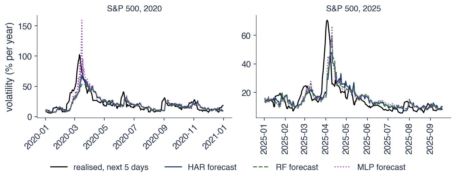
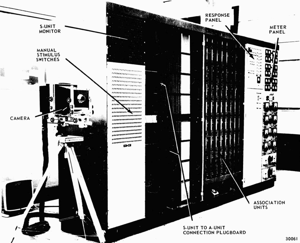

 SFM_ch13_validation