Bucharest University of Economic Studies IDA Institute Digital Assets Blockchain Research Center AI4EFin Artificial Intelligence for Energy Finance Romanian Academy, Institute for Economic Forecasting MSCA Digital Finance
A price level on its own says little about an investment. A share quoted at a few lei and an index quoted in thousands of points cannot be compared, and neither number shows how much an investor gained, how much the value fluctuated along the way or how deep the worst fall was. This chapter turns raw market data into numbers that do allow such comparisons: returns, measures of risk and drawdowns, together with their estimation error.
The chapter works throughout with real daily data for the BET index of the Bucharest Stock Exchange (BVB), the S&P 500, the DAX, Bitcoin and five BVB stocks, over the comparison period 2015–2026. The data already show the main themes of the course. Over this period 100 units invested in Bitcoin grew to 29,475, against 379 in the S&P 500, but Bitcoin's maximum drawdown was −83.4%. Daily returns have heavy tails: beyond three standard deviations the S&P 500 has 5.2 times as many days as the Normal distribution predicts. The annualised Sharpe ratio of the S&P 500, 0.72, has a standard error of 0.29, so most rankings of assets by such indicators are not statistically significant.
Before any statistic, the chapter deals with the quality of the data: the choice of the primary source, the adjustment of prices for dividends and splits, and the errors that real series contain.
Value of 100 units invested on the first day of 2015 in the S&P 500, the DAX, the BET and Bitcoin, on a logarithmic vertical axis: equal vertical distances correspond to equal percentage changes.
Learning outcomes
Choose a reliable data source and check a price series before using it.
Compute simple and log returns and aggregate them over time and across assets.
Annualise means and volatilities with the actual frequency of the data.
Describe a return series by its moments, quantiles and extreme values.
Compute and interpret the CAGR, the Sharpe and Sortino ratios, the maximum drawdown, the Calmar ratio and volatility drag.
Compare the difference between two indicators with their estimation error.
The student version of the seminar is available as a PDF.
Performance IndicatorsSharpe, Sortino, drawdown, Calmar and volatility drag, with their estimation error.
AI for Scientific DiscoveryAn open question on the persistence of Sharpe ratios and the checks an AI-assisted study needs.
SummaryThe formulas of the chapter and self-assessment questions.
Financial Data: Sources and Quality
Every result in this course starts from a data file, and every error in that file passes into the results. This section describes what financial data are, how often they are recorded, where they come from and which data the course uses. It then shows, on real series, the two operations that most often decide whether a price series can be used: the adjustment for corporate actions and the check against a second source. It ends with three systematic biases that leave no visible trace in the data but make results look better than they are.
Financial data fall into four groups. Market data are the information produced by a trading venue: trade prices, the best bid and ask quotes, traded volume, and derived series such as index levels, exchange rates, interest rates and crypto prices. The best bid is the highest price at which someone is willing to buy at a given moment, the best ask the lowest price at which someone is willing to sell; the gap between them, the spread, is the cost of an immediate round trip.
Corporate actions form a separate group because they change the quoted price without changing the value of an investor's holding. When a company pays a cash dividend, the share price falls on the ex-dividend day by roughly the amount paid, but the shareholder receives the cash. In a split, each old share becomes several new ones at a proportionally lower price; in a consolidation (reverse split) several old shares become one. Bonus shares work like a split. A series of quoted prices that ignores these events contains jumps that no investor experienced.
Fundamental and macroeconomic data, such as balance sheets, earnings, inflation, gross domestic product (GDP) and policy rates, describe the firms and the economy behind the prices. Alternative data include news, social media, satellite images and blockchain transactions. The course works mainly with daily market data.
In brief
Market data: what happens on a trading venue
trade prices, best bid and ask quotes, traded volume
index levels, exchange rates, interest rates, crypto prices
Corporate actions: events that change the price without changing the value of a holding
The first real-time price feed was the stock ticker, in use from 1867. The machine received trade prices by telegraph and printed them on a paper tape: the price of the last trade, a few minutes after it had taken place. Investors far from the exchange floor could follow the market almost as it happened.
Today exchanges publish electronic feeds that data vendors collect and redistribute. Every quote and every trade is recorded with a time stamp to the microsecond. Most statistical studies, including this course, do not use these records directly but their daily summaries, the OHLCV bars (open, high, low, close, volume) introduced below.
The tape survives in two forms. Moving bands of prices and news still run along building facades, such as the Reuters building in New York shown on the slide. The short ticker symbols that identify securities also come from the tape: at the BVB, TLV is Banca Transilvania, SNP is OMV Petrom and H2O is Hidroelectrica.
In brief
From 1867, stock tickers printed trade prices on a paper tape, sent by telegraph
the first real-time price feed: the price of the last trade, minutes after it happened
Today: electronic feeds from the exchanges, resold by data vendors
every quote and trade, time-stamped to the microsecond
daily summaries (OHLCV) are what most studies use
The ticker survived: scrolling prices and news on building fronts; ticker symbols such as TLV, SNP, H2O on the BVB
The finest level of data is tick data: every trade and every quote. A liquid market produces millions of records per day. Tick prices carry microstructure noise; the best-known source is the bid–ask bounce, in which successive trades execute alternately at the bid and at the ask, so that the trade price jumps back and forth even when the value of the asset does not change. Intraday bars, of 1, 5 or 60 minutes, summarise the ticks and are the input of realised volatility, the subject of Chapter 8.
Daily data, with one row per trading day, are the standard of this course and of most academic studies. Exchanges trade about 250 days per year, crypto markets 365 days per year, weekends and holidays included. Weekly, monthly and annual data give fewer observations but are closer to the horizon of a long-term investor.
The frequency matters for every annualised figure in this chapter. The rule is to annualise with the actual number of observations per year of each series, about 252 for an exchange and 365 for Bitcoin, never with a single factor for all assets. The consequences of using the wrong factor are shown in the section on annualisation.
In brief
Tick data: every trade and quote
millions of records per day; noise from the bid–ask bounce
The table on the slide lists six types of source. Exchanges (the BVB, Deutsche Börse, the New York Stock Exchange, NYSE) publish official prices, volumes and index levels, on their sites and through paid feeds. Data vendors such as Bloomberg, LSEG (the London Stock Exchange Group, formerly Refinitiv) and EODHD (EOD Historical Data, where EOD means end of day) gather prices from many markets, compute adjusted prices and add fundamental data, by subscription. Central banks, such as the National Bank of Romania (BNR), the European Central Bank (ECB) and the Federal Reserve, publish reference exchange rates and interest rates free of charge.
Statistical databases such as FRED (Federal Reserve Economic Data, from the Federal Reserve Bank of St. Louis) and Eurostat provide macroeconomic series and government bond yields. Academic databases such as CRSP (the Center for Research in Security Prices at the University of Chicago) and the Kenneth French data library provide cleaned returns, including those of delisted firms, and factor returns, under a university licence or free. Crypto exchanges and aggregators supply prices around the clock and on-chain data.
A vendor collects and cleans the data, but it is not the origin of the number. When two sources disagree, the reference is the primary source of the figure: the exchange for a closing price, the central bank for a reference exchange rate. The EUR/RON example shows why this rule matters.
In brief
Source
What it provides
Access
Exchanges (BVB, Deutsche Börse, NYSE)
official prices, volumes, index levels
website, paid feeds
Data vendors (Bloomberg, LSEG, EODHD)
prices from many venues, adjusted prices, fundamentals
subscription
Central banks (BNR, ECB, Federal Reserve)
reference exchange rates, interest rates
free
Statistical databases (FRED, Eurostat)
macro series, yields
free
Academic databases (CRSP, Kenneth French library)
cleaned returns, including delisted firms; factor returns
university licence or free
Crypto exchanges and aggregators
prices 24/7, on-chain data
free or subscription
A vendor collects and cleans; the primary source of a number (exchange, central bank) is the reference when two sources disagree
The course uses daily market data from EODHD, stored as a fixed snapshot so that every result can be reproduced. The collection holds 91 series: indices, exchange-traded funds (ETFs, funds traded on an exchange that track an index), stocks from the BVB, the US and Europe, crypto assets, exchange rates and bond yields. Each series has the same columns: date, open, high, low, close, adjusted close and volume.
The EUR/RON exchange rate is the exception. The course uses the official BNR reference rate, because the EODHD series for this rate contains erroneous quotes; the frame Data Errors: Two EUR/RON Series measures the damage.
Three conventions apply throughout. Indices, exchange rates and crypto assets use the close; stocks and ETFs use the adjusted close, so that dividends and splits are taken into account. Weekend quotes and repeated closes on holidays are removed, except for crypto assets, which trade every day. Each series is analysed on its own calendar, so the BET and the S&P 500 keep their own trading days. The comparison period of the chapter runs from 1 January 2015 to 18 September 2026.
In brief
Daily market data from EODHD (EOD Historical Data), saved once in the course repository
A daily bar records five numbers for day \(t\): the opening price \(O_t\), the highest price \(H_t\), the lowest price \(L_t\), the closing price \(C_t\) and the volume \(V_t\), the number of shares traded. By construction, the open and the close lie between the low and the high, \(L_t \le O_t, C_t \le H_t\). The range \(H_t - L_t\) measures how far the price moved during the day and is the basis of the range-based volatility estimators of Chapter 8.
The table shows the last five trading days of Banca Transilvania (TLV) in the course data, from 14 to 18 September 2026. Four of the rows look ordinary: the close moves between 33.40 and 35.50 lei and the volume between 346,819 and 1,884,988 shares. The bar of 17 September 2026 is different. Open, high, low and close are all equal to 33.40 lei, the same value as the close of the previous day, while the volume is 1,084,380 shares.
A flat bar is normal for an illiquid share on a day with a single trade, or for a holiday filled in with the previous price. With more than a million shares traded, a single price for the whole day is very unlikely, so the bar is suspect and has to be checked against the exchange. Simple checks of this kind, the inequalities between the four prices, flat bars and zero volumes, find many data errors before they reach any statistic.
In brief
OHLCV: open \(O_t\), high \(H_t\), low \(L_t\), close \(C_t\), volume \(V_t\) of day \(t\)
By construction \(L_t \le O_t, C_t \le H_t\); the range \(H_t - L_t\) measures the intraday spread of prices
Banca Transilvania (TLV), the last five trading days in our data:
Date
Open
High
Low
Close
Volume
14 Sep 2026
\(34.52\)
\(34.86\)
\(34.28\)
\(34.54\)
346 819
15 Sep 2026
\(34.40\)
\(34.68\)
\(33.10\)
\(34.00\)
676 653
16 Sep 2026
\(34.00\)
\(34.10\)
\(33.20\)
\(33.40\)
853 078
17 Sep 2026
\(33.40\)
\(33.40\)
\(33.40\)
\(33.40\)
1 084 380
18 Sep 2026
\(34.22\)
\(35.80\)
\(34.22\)
\(35.50\)
1 884 988
Check: on 17 September 2026 open = high = low = close with 1 084 380 shares traded; a flat bar with a large volume is suspicious
On the day of a corporate action the closing price \(P_t\) jumps, although the value of the holding does not change. The adjusted price removes these jumps. Each event \(k\), on day \(t_k\), has an adjustment factor\(F_{t_k}\). For a cash dividend \(D\),\(F = 1 - D/P_{t-1}\): the price falls by about \(D\) on the ex-dividend day, and scaling the earlier prices by \(F\) removes this fall. For an \(m\)-for-\(n\) split, in which \(n\) old shares become \(m\) new ones, \(F = n/m\); a consolidation is a split with \(m < n\), so its factor is greater than one and scales the earlier prices up.
The adjusted price multiplies each past price by the factors of all later events:
The product in (1.1) runs only over events after day \(t\), so the latest prices remain unchanged and the adjustment works backwards in time. Returns computed from adjusted prices include the dividend and contain no artificial jumps.
The same idea appears directly in the definition of the return. With a dividend \(D_t\) paid on day \(t\), the simple return is \(R_t = (P_t + D_t)/P_{t-1} - 1\)(Franke, Härdle & Hafner, 2019): the investor's gain is the change in price plus the cash received. A return computed from the adjusted close gives, up to a negligible second-order term, the same value.
In brief
The traded close \(P_t\) jumps on the day of a corporate action; the value of a holding does not
Adjustment factor\(F\) on the event day
cash dividend \(D\): \(F = 1 - D/P_{t-1}\)
split \(m\)-for-\(n\) (\(m\) new shares for \(n\) old): \(F = n/m\); a consolidation is a split with \(m < n\)
Adjusted close: every earlier price is multiplied by the factors of all later events, \(P^{\text{adj}}_t = P_t \prod_{k:\, t_k > t} F_{t_k}\)
\(t_k\): the day of event \(k\); the product runs over all events after day \(t\), so the last prices stay unchanged
returns computed from adjusted prices include the dividend and have no artificial jumps
With dividends, the simple return is \(R_t = (P_t + D_t)/P_{t-1} - 1\), with \(D_t\) the dividend paid on day \(t\)Franke, Härdle & Hafner (2019)
Consider a share quoted at 100 that pays a dividend of 2 on day 5 and has a 2-for-1 split on day 10. The dividend factor is \(F_5 = 1 - 2/100 = 0.98\) and the split factor \(F_{10} = 1/2 = 0.50\). A price before day 5 is followed by both events, so it is multiplied by \(0.98 \times 0.50 = 0.49\), and 100 becomes 49. A price between days 5 and 9 is followed only by the split and is multiplied by 0.50. From day 10 onwards no event follows, and the adjusted price equals the quoted price.
The example shows a property of the adjusted series that is easy to forget: it changes every time a new event occurs. After the next dividend, every earlier adjusted price is scaled again. Two downloads of the same adjusted series made at different dates therefore differ, and a result can be reproduced only if the download date is kept together with the data.
Indices face the same choice. A price index ignores dividends, so its level falls when the constituents go ex-dividend. A total return index reinvests the dividends in the index and measures what an investor holding the constituents would have earned. The BET and BET-TR comparison shows how large the difference becomes over a decade.
In brief
A share trades at 100; on day 5 it pays a cash dividend of 2; on day 10 it splits 2-for-1
Question for the room On the slide, the daily returns of the two series differ by more than 2 percentage points on 24 days since 2015. The ▶ button raises the threshold. How many days remain at a threshold of 10 percentage points?
Answer
11 days. Besides the consolidation of 16 August 2022 (+230.3% from the close, 0.0% from the adjusted close), 10 other days show a gap of more than 10 percentage points between the two log returns, all with the close falling; the largest, 19.5 percentage points, on 3 August 2017. Above 20 percentage points only the consolidation remains. A return computed from the close would treat these days as losses of the shareholders, although the value of the holding did not change.
The chart compares the two prices of Banca Transilvania on a logarithmic vertical axis: the close as traded (red) and the adjusted close (green). On 16 August 2022 the traded price jumps from 2.12 to 21.20 lei. Nothing happened to the value of the bank: it was a consolidation of the shares, ten old shares into one new share.
A log return computed from the traded close records this day as a gain of +230% in a single day, a number that would dominate any mean, variance or kurtosis of the series. Computed from the adjusted close, the return of the same day is 0.0%. Before August 2022 the adjusted price lies above the traded one, because the consolidation factor of 10 scales all earlier prices up; dividends and bonus shares, which scale earlier prices down, narrow the gap. At the end of the sample the two lines coincide, as (1.1) requires.
The consolidation is the most visible event but not the only one. Since 2015 the daily returns of the two series differ by more than 2 percentage points on 24 days, the days of dividends and bonus shares. Each of these days would add a spurious loss to a return series built from the traded price.
In brief
On 16 August 2022 the close jumps from 2.12 to 21.20 RON: a share consolidation, 10 old shares into one
Log return from the close: \(+230\%\) in one day; from the adjusted close: \(0.0\%\)
Since 2015 the daily returns of the two series differ by more than 2 percentage points on 24 days (dividends, bonus shares)
Question for the room The ▶ button moves the date of the investment from 2014 to 2025. With the investment made at the start of 2022, by how many percentage points a year does BET-TR grow faster than BET?
Answer
By 8.3 percentage points: 29.9% a year against 21.6%. The final values are 342 and 251, a gap of 91 units, much smaller than 1,005 against 455 for the investment of 23 September 2014. The gap between the growth rates, however, stays between 7.5 and 8.4 percentage points for every start year: dividends add roughly the same return every year, and their effect on wealth accumulates over time.
The BET (Bucharest Exchange Trading) index is the benchmark index of the BVB and a price index. The BET-TR (BET Total Return) has the same constituents but reinvests their dividends. The chart follows 100 units invested in each on 23 September 2014: at the end of the sample the investment is worth 455 in the BET and 1,005 in the BET-TR. The two lines start together and separate a little more each year, because each dividend reinvested in the BET-TR earns the later returns as well.
In annual terms, the growth rate is 13.5% per year for the BET and 21.2% for the BET-TR. Dividends add 7.8 percentage points per year, more than half of the growth of the price index. On the BVB, ignoring dividends gives a very incomplete picture of what an investor in the market earned.
The lesson applies to every comparison of indices: compare like with like. The DAX is a total return index, while the S&P 500 and the BET are price indices. A comparison of the DAX with the S&P 500 or with the BET therefore favours the DAX by the dividend yield of the other two markets. The tables later in the chapter include the BET-TR next to the BET for this reason.
In brief
100 invested on 23 September 2014: 455 in the BET (price index), 1 005 in the BET-TR (dividends reinvested)
Growth rate: 13.5% vs 21.2% a year; dividends add 7.8 percentage points a year
Compare like with like: the DAX is a total return index, the S&P 500 and the BET are price indices
Question for the room The annualised volatility of the EODHD series is 13.4%, that of the BNR rate 4.5%. What does the volatility of the EODHD series become if we drop the 412 days on which the daily changes differ by more than 1 percentage point, that is 8% of the days?
Answer
About 4.7%, close to 4.3%, the volatility of the BNR rate on the same days. Volatility depends on squared deviations, so a few hundred wrong quotes triple it. Of the 412 days, 307 fall in 2010–2013. 283 days differ by more than 2 percentage points, 10 days by more than 5 percentage points.
The chart plots the daily log returns of two series of the same exchange rate, EUR/RON: the series from EODHD (red) and the BNR reference rate (green). The two series have 5,154 days in common. On 412 of them, the daily change of the EODHD series differs from that of the BNR rate by more than 1 percentage point, a very large difference for an exchange rate whose genuine daily changes are usually a small fraction of a percent. The red series shows a block of alternating erroneous quotes between about 2010 and 2014 and isolated spikes of more than 10% in both directions.
The errors change every statistic. The annualised volatility of the EODHD series is 13.4%, against 4.5% for the BNR rate. The largest daily change of the EODHD series, in absolute value, is 15.4%, on 14 August 2025: it is the return to the correct level after a wrong quote on the previous day. A single bad quote thus produces two extreme returns of opposite sign, the error and its reversal, and both inflate the volatility and the kurtosis.
The solution is the rule of the sources frame: use the primary source of the figure. For a reference exchange rate the primary source is the central bank, and the course uses the BNR series. An error of this kind is found by comparing two sources, or by listing the largest returns and checking each of them.
In brief
Same exchange rate, 5 154 common days: the EODHD series moves by more than 1 percentage point more than the BNR rate on 412 days
Annualised volatility: 13.4% (EODHD) vs 4.5% (BNR); largest absolute EODHD move \(15.4\%\) on 14 August 2025, the reversal of a wrong quote of the previous day
Fix: use the primary source of the number, the BNR reference rate
Some errors do not lie in individual prices but in the way the sample is chosen or used. Survivorship bias arises when the sample contains only the firms or funds that still exist. Firms with poor results were delisted, merged or went bankrupt, so they are missing, and the average return of the survivors overstates what an investor could have earned (Brown et al., 1992). An example is the current composition of the BET traced back to 2000: the companies that left the index in the meantime are not in the sample.
Look-ahead bias is the use of information that was not available at the date of the decision. A typical case is an annual report published in March and used in a backtest for decisions taken in January. The backtest then trades on numbers the investor could not yet know. Database dates often record the period to which a figure refers, not the date of its publication, which makes this error easy to commit.
Data snooping is trying many rules on the same data and reporting the best one. Even if no rule works, the best of many looks significant by chance. Harvey, Liu & Zhu (2016) conclude that hundreds of published predictors of returns are probably false discoveries. All three biases overstate returns, and none of them shows up in the descriptive statistics of the final sample, which look perfectly normal. They can only be prevented by the design of the study.
In brief
Survivorship bias: only firms or funds that still exist are in the sample
the losers have disappeared, so the average return is too high Brown et al. (1992)
example: today's members of the BET, followed back to 2000
Look-ahead bias: using information not yet available at the decision date
annual reports published in March used for decisions in January
Data snooping: trying many rules on the same data and reporting the best one
The errors of this section can be caught by a short routine applied to every new series. First, record the source: the primary source of the figure and the column used, close or adjusted close. Second, check the calendar: weekends, holidays and missing days, and, in a joint analysis of several assets, the same dates for all of them.
Third, look for jumps: list the 10 largest returns in absolute value and check each against the news of that day. A genuine crash has a known cause; a consolidation or a wrong quote does not. Fourth, look for flat bars, zero volume and repeated prices, which reveal holidays filled in with the last price or stale prices, quotes that were not updated. Fifth, check units and currency: lei, euro or dollars, index points, prices quoted in cents.
Finally, keep the raw file and the download date, and never edit the data by hand. Every correction is made in code, where it can be read, repeated and reversed. These rules cost little and protect every later result of the course.
In brief
Source: the primary source of the number and the column used (close or adjusted close)
Calendar: weekends, holidays, missing days; same dates for all assets in a joint analysis
Jumps: list the 10 largest absolute returns and check each against the news
Flat bars, zero volume, repeated prices: holidays filled with the last price or stale quotes
Units and currency: RON, EUR, USD; index points; prices in cents
Keep the raw file and the download date; never edit data manually
Prices come from exchanges, data vendors and central banks, and when sources disagree the primary source of the figure is the reference. For stocks the adjusted price must be used, and when dividends matter, as on the BVB, total return indices must be used instead of price indices: over 2014–2026 the BET-TR grew to 1,005 from an initial 100, the BET only to 455.
Real data contain errors, such as the ten-to-one consolidation of Banca Transilvania or the wrong quotes of the EODHD EUR/RON series. They are found by checking jumps, flat bars and a second source. Survivorship bias, look-ahead bias and data snooping overstate results without leaving any visible trace in the data.
In brief
Prices come from exchanges, vendors and central banks; the primary source of a number is the reference
Use adjusted prices for stocks, total return indices when dividends matter
Real data contain errors: check jumps, flat bars and a second source
Survivorship, look-ahead and data snooping inflate results silently
Section summary
A usable price series is the end of a chain of decisions: the source, the column, the calendar, the adjustment for corporate actions and the checks for errors. The examples of the section show that each link matters: one consolidation produces a fictitious one-day return of +230%, ignoring dividends removes 7.8 percentage points per year from the growth of the Romanian market, and a series with wrong quotes triples the volatility of an exchange rate. With clean prices in hand, the next section explains why the statistics of the course work with returns rather than prices.
From Prices to Returns
The statistical methods of this course are applied to returns, not to prices. This section gives the reasons: returns have no unit, so they can be compared across assets, and they fluctuate around a stable level, while prices follow a trend. The second property is made precise by the notion of weak stationarity and checked formally with the augmented Dickey–Fuller (ADF) test on the S&P 500.
A price has a unit and a scale; a return has neither. A change of 1 leu is large for a share quoted at 2 lei and small for one quoted at 500 lei. A return expresses the change relative to the starting price, so returns of different assets, in different currencies and over different periods can be compared directly. The investor's question is also relative: by how much did my wealth change? That is exactly a return.
The second reason is statistical. Prices follow a trend and do not return to a fixed level, so their mean and variance depend on the period observed. Returns fluctuate around a stable level. The concept behind this distinction is weak stationarity: a series is weakly stationary if its mean is constant, its variance is constant and the covariance between two observations depends only on the distance between them, the lag, not on the date.
Most statistical methods of the course assume at least weak stationarity, because only then can averages over time estimate fixed population quantities. A sample mean of prices estimates nothing stable; a sample mean of returns estimates the expected return. The next two frames show the difference on data and test it formally.
In brief
A price has a unit and a scale; a return does not
a 1-leu move is large for a 2-leu share and small for a 500-leu share
Returns of different assets, currencies and periods can be compared directly
Prices trend and wander; returns fluctuate around a stable level
weakly stationary series: constant mean, constant variance, and a covariance that depends only on the lag
most statistical methods of this course assume (at least) weak stationarity
The investor cares about the relative change of wealth, which is exactly a return
Question for the room The ▶ button splits the 2000–2026 sample into up to 6 equal subperiods. With 5 subperiods, what happens to the mean and the standard deviation of daily returns from one subperiod to the next?
Answer
The mean of returns stays close to zero, between −0.016% and 0.057% a day, while the mean of the price rises from 1,145 to 5,235 points. The standard deviation of returns, however, varies between 0.97% and 1.53% a day: returns fluctuate around a stable level, but their volatility changes over time. The ADF test rejects the unit root for returns (statistic −14.3), not for the log price (statistic −2.08, p-value 0.56).
The upper panel shows the S&P 500 in index points since 2000. The price has an upward trend with long swings: the falls of 2000–2002 and 2008–2009 and a strong rise after 2012. Its mean and dispersion over any window depend on which years the window covers, which is what non-stationarity means in practice.
The lower panel shows the daily log returns of the same index. They fluctuate around zero over the whole period, in calm years and in turbulent ones, such as the financial crisis of 2008 and the pandemic shock of 2020. The level of the series does not drift.
The lower panel also shows that the size of the fluctuations is not the same at all times: large returns come in clusters, around 2008 and 2020. This phenomenon, volatility clustering, does not contradict weak stationarity, which concerns the unconditional variance. A series can have a constant long-run variance while its variance conditional on the recent past changes from day to day. The models that describe this are the subject of Chapter 9.
In brief
Top: the price trends upward with long swings; its mean and spread change over time
Bottom: the returns fluctuate around zero, in calm and turbulent periods (2008, 2020)
The augmented Dickey–Fuller (ADF) test (Dickey & Fuller, 1979) asks whether a series has a unit root, that is, whether it behaves like a random walk. The null hypothesis \(H_0\) is a unit root, so the series is non-stationary; the alternative \(H_1\) is that the series is stationary. The test regresses the daily change of the series on its level on the previous day:
In (1.2),\(y_t\) is the series tested, the log price or the log return, and \(\Delta y_t = y_t - y_{t-1}\) is its change from day \(t-1\) to day \(t\). The constant \(\alpha\) and the linear trend \(\beta t\) allow for drift and trend; the \(p\) lagged changes, with coefficients \(\delta_j\), absorb short-term autocorrelation, and \(\varepsilon_t\) is the error. The key coefficient is \(\gamma\). If \(\gamma = 0\), today's change does not depend on yesterday's level: the series has no level to return to, which is a unit root. If \(\gamma < 0\), a high level is followed on average by a fall and a low level by a rise, so the series is pulled back towards its level and is stationary.
The test rejects \(H_0\) when the \(t\) statistic of \(\hat\gamma\) lies below a critical value. The critical values do not come from the Student distribution but from the Dickey–Fuller tables, because under \(H_0\) the regressor \(y_{t-1}\) is itself non-stationary and the \(t\) statistic has a non-standard distribution, shifted to the left. The critical value also depends on whether the constant and the trend are included.
In brief
ADF test (augmented Dickey–Fuller) Dickey & Fuller (1979): is there a unit root (a random walk) in the series?
\(H_0\): unit root, the series is non-stationary; \(H_1\): the series is stationary
The test regresses the daily change of the series on its previous level
\(y_t\): the tested series (log price or log return); \(\Delta y_t = y_t - y_{t-1}\): its change from day \(t-1\) to day \(t\)
\(\alpha\): constant; \(\beta t\): linear trend; \(\delta_j\): coefficients of the \(p\) lagged changes, which absorb short-term autocorrelation; \(\varepsilon_t\): error
\(\gamma = 0\): the series does not return to a level (unit root); \(\gamma < 0\): it is pulled back (stationary)
Reject \(H_0\) when the \(t\)-statistic of \(\hat\gamma\) is below the critical value (Dickey–Fuller tables, not Student)
On daily S&P 500 data since 2000, the test gives two clear answers. For the log price, with a trend in the regression, the statistic is −2.08, the 5% critical value is −3.41 and the p-value is 0.56: the unit root is not rejected. For the log returns, the statistic is −14.3, the 5% critical value is −2.86 and the p-value is below 0.001: the unit root is rejected. The two critical values differ because the first regression includes a trend and the second only a constant.
The p-value is the probability, under \(H_0\), of obtaining a statistic at least as negative as the one observed. A p-value of 0.56 means that a random walk would produce a statistic like −2.08 more than half of the time, so the data give no reason to doubt the unit root. A statistic of −14.3 is practically impossible under a unit root. With the usual threshold of 0.05, \(H_0\) is rejected for returns and kept for prices.
The conclusion supports the choice of the course: prices behave like a random walk, returns are stationary, so the statistical models are built for returns. Failing to reject a unit root does not prove that one exists, but the two results together give a consistent picture. Unit roots and the random walk hypothesis are studied in detail in Chapter 7.
In brief
S&P 500, daily data since 2000
log price (with trend): statistic \(-2.08\), 5% critical value \(-3.41\), p-value \(0.56\): we do not reject the unit root
log returns: statistic \(-14.3\), 5% critical value \(-2.86\), p-value \(< 0.001\): we reject it
Reading
p-value: the probability, under \(H_0\), of a statistic at least as negative as the observed one; below 0.05 we reject \(H_0\)
prices behave like a random walk; returns are stationary, so we model returns, not prices
Unit roots and random walks are the subject of Chapter 7
Returns are preferred to prices for two reasons: they have no unit, so they can be compared across assets and periods, and they are stationary while prices are not. On the S&P 500 since 2000, the ADF test keeps the unit root for the log price (statistic −2.08, p-value 0.56) and rejects it for the log returns (statistic −14.3). There are, however, two ways to define a return, and the next section shows when they differ and which one to use.
Simple and Log Returns
A return can be defined as a relative change of the price or as the change of its logarithm. The two definitions give almost the same number for a typical day and very different numbers for a crash or over a long horizon. This section defines both, measures the gap between them, illustrates it on the most extreme days of Bitcoin and the S&P 500, and gives a rule for choosing between them.
The ratio \(1 + R_t = P_t/P_{t-1}\) is the gross return: the value at \(t\) of one unit invested at \(t-1\). From here on, \(P_t\) denotes the closing price of an index or the adjusted price of a stock, so that dividends and splits are already taken into account.
The simple return is bounded below: \(R_t \ge -1\). The bound expresses limited liability: the price cannot fall below zero, so a shareholder cannot lose more than the amount invested. For example, with \(P_{t-1} = 100\) and \(P_t = 110\),\(R_t = 10\%\). This is the number an investor sees on an account statement when the fund reports that it "gained 10%".
The name comes from compounding. One leu invested at a rate \(r\) compounded \(m\) times during the period grows to \((1 + r/m)^m\), and as \(m \to \infty\) this tends to \(e^{r}\). The log return is therefore the rate that, compounded continuously over the period, turns \(P_{t-1}\) into \(P_t\). With \(P_{t-1} = 100\) and \(P_t = 110\),\(r_t = \ln 1.1 = 9.53\%\), below the simple return of 10% on the same prices.
Unlike the simple return, the log return is unbounded: \(r_t \in (-\infty, +\infty)\), and a total loss, \(P_t = 0\), corresponds to \(r_t = -\infty\). Log returns are the default in the statistics of financial markets. The main reason, shown in the next section, is that they add up over time, so that the return over a long period is the sum of the daily returns. Their range over the whole real line also suits statistical models better.
The logarithm is concave, so its graph lies below its tangent at zero, the line \(r = R\). Hence \(r < R\) for every \(R \neq 0\), for gains as well as for losses. For small changes the first correction term, \(-R^2/2\), gives almost the whole gap.
For a typical daily change of \(R = 1\%\),\(r = 0.995\%\), and the approximation \(R - R^2/2\) also gives 0.995%. The gap \(R - r\) is 0.5 basis points; a basis point (bp) is 0.01 percentage points. For a large change of \(R = 10\%\),\(r = 9.531\%\), while \(R - R^2/2 = 9.500\%\), and the gap \(R - r\) is 46.9 basis points. For daily data the two returns are practically equal; for large changes and long horizons they differ, and the gap grows with the square of the change.
Question for the room Bitcoin, 7 December 2017: R = +25.2%, r = +22.5%, so R − r = 2.7 percentage points. What is the gap R − r for a fall of the same size, R = −25.2%?
Answer
3.8 percentage points: r = ln(0.748) = −29.0%. The function ln is concave, and the gap is larger for falls than for rises of the same size. The approximation R²/2 = 3.2 percentage points is the same for both signs; the R³/3 term of the Taylor series corrects it upwards for falls and downwards for rises. At R = −37.2% (Bitcoin, 12 March 2020), the gap reaches 9.3 percentage points.
The chart plots the log return against the simple return. The dashed line is the 45-degree line \(r = R\), the solid curve is \(r = \ln(1 + R)\), and the markers are the largest daily moves of Bitcoin (circles) and of the S&P 500 (squares). Near zero the curve and the line coincide; away from zero the curve lies below the line on both sides, and the gap grows much faster on the side of losses.
The largest daily moves in the course data show the size of the gap. On 12 March 2020 Bitcoin had a simple return of −37.2% but a log return of −46.5%. On 7 December 2017 it had a simple return of +25.2% and a log return of +22.5%. On 16 March 2020 the S&P 500 had a simple return of −12.0% and a log return of −12.8%.
Because the curve is concave, losses look larger and gains look smaller when measured in log returns. The asymmetry has a precise meaning: a log return of −46.5% and one of +46.5% cancel exactly, while a simple loss of 37.2% needs a simple gain of much more than 37.2% to be recovered. On days like these the choice of return changes the number reported by several percentage points.
In brief
Bitcoin, 12 March 2020: \(R = -37.2\%\) but \(r = -46.5\%\)
Bitcoin, 7 December 2017: \(R = +25.2\%\), \(r = +22.5\%\)
Consider the price path \(100 \to 110 \to 99\). The simple returns are \(+10\%\) and \(-10\%\), and their sum, zero, suggests that the investor is back where they started. The investor has in fact lost: compounding the two returns gives \(1.1 \times 0.9 - 1 = -1.0\%\), the change from 100 to 99.
The log returns of the same path are \(r_1 = \ln 1.1 = 9.53\%\) and \(r_2 = \ln 0.9 = -10.54\%\). Their sum is \(-1.01\%\), which equals \(\ln(99/100)\) exactly. Adding log returns gives the correct two-period log return without any correction.
The rule that follows is the main practical difference between the two returns: simple returns compound, that is, gross returns multiply, while log returns add. A gain and a loss of the same size in percent do not cancel; in simple returns the loss of 10% applies to a larger base than the gain of 10%.
In brief
Price path \(100 \to 110 \to 99\)
simple returns: \(+10\%\) and \(-10\%\); their sum, 0, is misleading
The question pushes the previous example to larger numbers. A share rises by 50% in one year and falls by 50% in the next. What does the price reach after two years, relative to its initial level?
Compounding the gross returns gives \(1.5 \times 0.5 = 0.75\): wealth has changed by −25%, although the two percentages have the same size. In log returns, \(\ln 1.5 + \ln 0.5 = \ln 0.75 = -28.8\%\), a direct sum.
The general form of the result is the recovery rule. After a loss \(x\), wealth is \(1 - x\) times its previous level, and returning to that level requires a gain of \(x/(1 - x)\). A loss of 50% therefore requires a gain of 100%. The required gain grows faster than the loss, which is why the depth of a fall matters so much in the drawdown measures of the chapter.
In brief
A share gains 50% one year and loses 50% the next
What do you think? Where is the price after two years, relative to the start?
Answer
\(1.5 \times 0.5 = 0.75\): the wealth changed by \(-25\%\)
The table on the slide matches each situation with a return. For aggregation over time, log returns are used, because the \(k\)-period log return is a sum, \(r_t(k) = r_t + \dots + r_{t-k+1}\). For a portfolio of several assets, simple returns are used, because the portfolio return is exactly the weighted average \(R_p = \sum_i w_i R_i\). For statistical modelling, log returns are preferred, because they are unbounded and their distribution is closer to symmetric.
For reporting to investors, the simple return is used, since "the fund gained 10%" is a simple return. For daily data and small changes either return will do, because the difference is about \(R^2/2\), half a basis point for a 1% day.
Whatever the choice, the type of return has to be stated. A "return of 10%" is ambiguous: as a log return it corresponds to a simple return of \(e^{0.1} - 1\), about 10.5%. On a single day the ambiguity costs little; over a decade, or for a volatile asset such as Bitcoin, it can change conclusions.
In brief
Task
Use
Reason
Aggregating over time
log
\(r_{t}(k) = r_t + \dots + r_{t-k+1}\), a sum
Portfolio of several assets
simple
\(R_p = \sum_i w_i R_i\), exact
Statistical modelling
log
unbounded, closer to a symmetric distribution
Reporting to investors
simple
“the fund gained 10%” is a simple return
Daily data, small moves
either
the difference is about \(R^2/2\)
Always say which one you use: a “return of 10%” is ambiguous
The simple return is \(R_t = P_t/P_{t-1} - 1\) and the log return \(r_t = \ln(P_t/P_{t-1}) = \ln(1 + R_t)\). For every non-zero change \(r < R\), and the difference is approximately \(R^2/2\), negligible for daily data and large for crashes, as on 12 March 2020, when Bitcoin fell by 37.2% in simple terms and by 46.5% in log terms.
Log returns add up over time; simple returns add up across assets. Gains and losses of the same size do not cancel: +50% followed by −50% leaves 75% of the initial wealth.
\(r < R\) for every move; the gap is about \(R^2/2\), negligible for daily data
Log returns add over time; simple returns add across assets
Gains and losses of the same size do not cancel
Section summary
The two returns carry the same information but behave differently under aggregation. Log returns (1.4) add over time and are the natural input of statistical models; simple returns (1.3) average exactly across assets and are what investors see. The gap, about \(R^2/2\), is 0.5 basis points on a 1% day and 9.3 percentage points on Bitcoin's worst day. The next section uses both properties to build returns over several periods and returns of portfolios.
Multi-Period and Portfolio Returns
Investors hold assets for months or years and usually hold several of them. This section builds the return over \(k\) periods from daily returns, links cumulative returns to wealth, and computes the return of a portfolio. The two aggregation rules of the previous section, sums over time for log returns and weighted averages across assets for simple returns, are applied to real data: four markets over 2015–2026 and a portfolio of two BVB stocks.
Both identities in (1.6) follow from writing \(P_t/P_{t-k}\) as a product of \(k\) one-period ratios; taking logarithms turns the product into a sum. Here \(R_t(k)\) and \(r_t(k)\) denote the simple and the log return over the \(k\) periods.
The additivity of log returns has an important consequence: the mean and the variance of the \(k\)-day log return follow from those of the daily returns. The mean of a sum is the sum of the means, so the \(k\)-day mean is \(k\) times the daily mean; if the daily returns are uncorrelated, the variance of the sum is also \(k\) times the daily variance. This is the basis of the annualisation rules of the next section but one.
Weekly, monthly or annual returns are computed from the prices at the end of each period, not by averaging the daily returns within it. The average of 21 daily returns is a daily figure, not a monthly return; the monthly log return is the sum of the daily ones, or equivalently the log of the ratio of the two month-end prices.
where \(\prod_{t=1}^{T}\) is the product of the \(T\) gross returns and \(\exp(x) = e^x\) inverts the logarithm. The two forms in (1.7) are the two identities of (1.6) applied over the whole sample.
The cumulative simple return\(\text{CSR}_T = W_T/W_0 - 1\) is the investor's gain in percent. The cumulative log return\(\text{CLR}_T = \ln(W_T/W_0) = \sum_t r_t\) is the sum of the log returns, and the two are linked by \(\text{CSR}_T = e^{\text{CLR}_T} - 1\). The cumulative log return is the natural scale for long horizons: it grows linearly when the growth rate is constant, while the cumulative simple return grows exponentially.
This explains why wealth charts use a logarithmic vertical axis. On a log scale, equal vertical distances correspond to equal percentage changes: a doubling from 100 to 200 and one from 1,000 to 2,000 have the same height. A constant growth rate appears as a straight line, and the slope of the line is the log growth rate.
In brief
Wealth after \(T\) periods, starting from \(W_0\): \(W_T = W_0 \prod_{t=1}^{T} (1 + R_t) = W_0 \exp\Big(\sum_{t=1}^{T} r_t\Big)\)
\(\prod_{t=1}^{T}\): the product of the \(T\) gross returns; \(\exp(x) = e^x\) undoes the logarithm
Question for the room With equal weights, the weighted sum of log returns gives a cumulative log return of 2.47 instead of 2.56. The ▶ button moves the TLV weight from 10% to 90%. At which weight is the gap between the two cumulative returns largest?
Answer
At 50%: 0.093. At 25% and 75% the gap is about 0.07, at 10% and 90% only 0.033. The daily gap is about w(1 − w)(RTLV − RSNP)²/2, largest for equal weights and zero for a single stock. The largest daily gap, 13.9 basis points on 31 May 2016, covers three trading days: SNP has no prices on 27 and 30 May 2016, so both returns run from 26 May; TLV rises by 6.6%, SNP falls by 4.0%.
Annualised volatility (%) by frequency of the log returns
Worked example: annualising the mean and the volatility
Question for the room From daily returns, the annualised volatility of the S&P 500 over 2015–2026 is 17.7%. The ▶ button switches to weekly and monthly returns. What does √12 × σ computed from the monthly returns give?
Answer
15.0%; from weekly returns, 16.7%. The square-root-of-time rule assumes uncorrelated returns with constant variance, and the S&P 500 does not follow it exactly over 2015–2026. The monthly series has only 140 returns, so its estimate also has a larger error. For Bitcoin the three values are close: 66.7%, 66.7% and 66.3%.
Annual mean of the daily log returns and its precision
Worked example: the standard error of the annual mean
Question for the room Over 2015–2026 (11.7 years), the 95% confidence interval of the annual mean of the S&P 500 is [1.1%; 21.4%]. The ▶ button moves the start of the sample. With the start in 2020 (6.7 years), does the interval contain 0?
Answer
Yes: 12.7% ± 15.3%, that is [−2.6%; 28.1%]. The estimated mean is higher than over 2015–2026, but the standard error rises from 5.2% to 7.8%, roughly as 1/√Y. The 1,686 daily returns do not help: the precision of the mean depends on the number of years. An interval that contains 0 does not show that the mean is zero, only that 6.7 years of data do not separate it from noise.
Question for the room The ▶ button moves the date of the investment from 2015 to 2025. With the investment made at the start of 2022, which of the four series has the largest final value?
Answer
BET: 251, against Bitcoin 170, S&P 500 161 and DAX 159. For the investment of 2015, Bitcoin reaches 29,475, and for that of 2018 592, still first. The ranking by cumulative return depends on the start date.
The chart follows 100 units invested on 5 January 2015, the first day of 2015 on which all four series have prices, on a logarithmic vertical axis. The CAGR tables later in the chapter start each series on its own first trading day of 2015, so their growth rates differ slightly from those implied by this chart: 11.9% against 12.0% for the S&P 500, 60.6% against 62.5% for Bitcoin. At the end of the sample the investment is worth 379 in the S&P 500, 267 in the DAX, 470 in the BET and 29,475 in Bitcoin. The DAX is a total return index while the S&P 500 and the BET are price indices, so the first three lines do not compare like with like, as noted for the BET and BET-TR.
For Bitcoin, the cumulative simple return is 29,375% and the cumulative log return is 5.69; for the BET, the two figures are 370% and 1.55. The pairs show the different scales of the two measures: a cumulative simple return of tens of thousands of percent corresponds to a cumulative log return of less than six, and the relation \(\text{CSR}_T = e^{\text{CLR}_T} - 1\) links them in both cases.
The logarithmic axis is what makes the chart readable. On a linear axis Bitcoin's line would rise to almost 30,000 and all the other series would appear as flat lines near the bottom. On the log axis the common shock of March 2020 is visible in all four series, as are Bitcoin's rise in 2017 and its fall in 2018.
In brief
100 invested on 5 January 2015, the first day with prices for all four series (the CAGR tables start each series on its own first day of 2015); final values: S&P 500 379, DAX 267, BET 470, Bitcoin 29 475
A portfolio holds \(n\) assets with weights \(w_1, \dots, w_n\),\(\sum_i w_i = 1\), fixed at the start of the period, where \(w_i\) is the share of wealth invested in asset \(i\). Let \(R_i\) and \(r_i\) be the simple and the log return of asset \(i\) over the period. Since wealth is additive across assets, the value of the portfolio at the end of the period is \(\sum_i w_i (1 + R_i)\) times its initial value, and the portfolio return is exactly the weighted average of the simple returns:
The log return of the portfolio, in (1.8), is the logarithm of a weighted sum and not a weighted sum of logarithms. For example, with 60% in asset 1, with \(R_1 = 10\%\), and 40% in asset 2, with \(R_2 = -5\%\), the portfolio return is \(R_p = 0.6 \times 10\% + 0.4 \times (-5\%) = 4.0\%\), and the exact portfolio log return is \(r_p = \ln(1 + R_p) = 3.92\%\). The weighted log returns give \(0.6 \times 9.53\% + 0.4 \times (-5.13\%) = 3.67\%\), which is too small. For weights between zero and one the weighted log return is always too small, by the convexity of the exponential (Jensen's inequality).
The weights do not stay fixed. When one asset rises more than the other its share of wealth grows, so a portfolio with fixed weights has to be rebalanced, by selling part of the winners and buying the losers. The formula \(R_p = \sum_i w_i R_i\) uses the weights at the start of each period, so a portfolio that is rebalanced daily applies it day by day.
In brief
Portfolio with weights \(w_1, \dots, w_n\), \(\sum_i w_i = 1\), set at the start of the period
\(R_i\), \(r_i\): the simple and the log return of asset \(i = 1, \dots, n\) over the period; \(w_i\): the share of wealth in asset \(i\)
The portfolio holds 50% Banca Transilvania (TLV) and 50% OMV Petrom (SNP), rebalanced daily, over 2015–2026. Each day it is possible to compare the exact portfolio log return, \(\ln(1 + R_p)\), with the weighted sum of the two log returns. The gap is small: its mean in absolute value is 0.38 basis points, and its largest value is 13.9 basis points, on 31 May 2016.
Over the whole period the small daily gaps accumulate, and always in the same direction. The exact cumulative log return of the portfolio is 2.56, so 1 leu becomes 13.0 lei. The weighted log returns give a cumulative log return of 2.47, which corresponds to only 11.8 lei. The error of more than one leu out of thirteen arises entirely from summing an approximation that is very accurate on a single day.
The growth rate of the portfolio is 24.5% per year, against 27.3% for TLV and 19.7% for SNP. The rule is therefore to build portfolios with simple returns, using (1.8), and to convert to log returns afterwards if needed, with \(r_p = \ln(1 + R_p)\).
In brief
50% Banca Transilvania, 50% OMV Petrom, rebalanced daily, 2015–2026
One day: exact log return vs weighted sum of log returns
mean absolute gap 0.38 basis points; largest gap 13.9 basis points, on 31 May 2016
Over the whole period the small gaps accumulate
exact cumulative log return 2.56, so 1 leu grows to 13.0 lei
weighted log returns give 2.47, so only 11.8 lei
Growth rate: portfolio 24.5% a year; TLV 27.3%; SNP 19.7%
Rule: build portfolios with simple returns, then take logs if needed
Over time, gross simple returns multiply and log returns add. Wealth follows \(W_T = W_0 e^{\text{CLR}_T}\), and the cumulative simple return is \(\text{CSR}_T = e^{\text{CLR}_T} - 1\), as for Bitcoin's 29,375%, which corresponds to a cumulative log return of 5.69.
Across assets, \(R_p = \sum_i w_i R_i\) is exact, while the weighted sum of log returns is only an approximation. Its daily error is tiny, 0.38 basis points on average for the TLV–SNP portfolio, but over a decade it becomes visible: 11.8 lei instead of 13.0.
In brief
Over time: multiply gross returns or add log returns
Across assets: \(R_p = \sum_i w_i R_i\) exactly; the log version is only an approximation
Small daily approximation errors become visible over a decade
Section summary
The section has fixed the two aggregation rules of the course: log returns for sums over time (1.6), simple returns for averages across assets (1.8). Wealth is the exponential of the cumulative log return (1.7), which is why long histories are plotted on a logarithmic axis. Investors, however, compare assets per year, not per day or per decade. The next section converts daily statistics into annual ones and measures how precisely the annual mean can be known.
Annualisation
Statistics computed from daily data are daily figures, while returns and risks are usually quoted per year. This section gives the rules for annualising the mean and the volatility, defines the compound annual growth rate (CAGR) and shows that, unlike volatility, the mean return is estimated very imprecisely, however frequent the data.
Let \(A\) be the number of observations per year: about 252 for an exchange, 365 for crypto, 52 for weekly data and 12 for monthly data. Let \(\mu\) and \(\sigma\) be the mean and the standard deviation of the returns at the frequency of the data, for example daily. Since log returns add up over a year, the annual mean is the sum of \(A\) daily means, and the same rule is used for the mean of simple returns, as an arithmetic annualisation. The volatility, the standard deviation of the returns, scales with the square root of \(A\):
The second rule in (1.9) is the square-root-of-time rule. It holds when the returns are uncorrelated and have constant variance: then \(\Var(r_1 + \dots + r_A) = A\,\sigma^2\), because all the covariances vanish, and the square root gives \(\sqrt{A}\,\sigma\). With positive autocorrelation the annual variance is larger than \(A\sigma^2\), and with negative autocorrelation smaller; this is the idea behind the variance ratio tests of Chapter 7.
For the S&P 500, the daily standard deviation is 1.12%, so the annual volatility is \(1.12\% \times 15.87 = 17.7\%\), where \(15.87 = \sqrt{252}\). For Bitcoin, which trades every day, the factor is \(\sqrt{365} = 19.10\), which gives 66.7%. The exchange factor \(\sqrt{252}\) would give only 55.4% and understate Bitcoin's risk by more than 11 percentage points. This is why the frequency rule of the data section matters.
In brief
\(A\) = number of observations per year: about 252 for exchanges, 365 for crypto, 52 for weekly, 12 for monthly data
\(\mu\), \(\sigma\): the mean and the standard deviation of the returns at the frequency of the data (for example, daily)
Mean: log returns add, so \(\mu_{\text{year}} = A\,\mu\)
the same rule is used for the mean of simple returns (arithmetic annualisation)
Volatility = standard deviation of returns: \(\sigma_{\text{year}} = \sqrt{A}\,\sigma\), the square-root-of-time rule
valid when returns are uncorrelated with constant variance: then \(\Var(r_1 + \dots + r_A) = A\,\sigma^2\), and the square root gives \(\sqrt{A}\,\sigma\)
The CAGR (compound annual growth rate) is the constant annual rate that turns the first price \(P_0\) into the last price \(P_T\) in \(Y\) years:
\[\text{CAGR} = \big(P_T / P_0\big)^{1/Y} - 1 ,\]
(1.10)
with \(Y\) measured in calendar years. Taking logarithms of (1.10) gives \(\ln(1 + \text{CAGR}) = \ln(P_T/P_0)/Y\), the cumulative log return per year. Hence \(\text{CAGR} = \exp(\text{annual mean of log returns}) - 1\).
For the S&P 500 over 2015–2026, the annual mean of the log returns is 11.2%, and \(e^{11.2\%} - 1 = 11.9\%\), the same value as the CAGR, 11.9%. The CAGR is also called the geometric mean return, because \(1 + \text{CAGR}\) is the geometric mean of the annual gross returns.
The CAGR uses only the first and the last price. It says nothing about the path between them: two investments with the same CAGR can have had very different volatilities and very different falls along the way. The indicators of the performance section measure these differences.
In brief
CAGR (compound annual growth rate): the constant yearly rate that turns \(P_0\) into \(P_T\) in \(Y\) years
\(\text{CAGR} = \big(P_T / P_0\big)^{1/Y} - 1\), with \(Y\) in calendar years
Link with log returns: \(\text{CAGR} = \exp(\text{annual mean log return}) - 1\)
S&P 500, 2015–2026: mean log return 11.2% a year, \(e^{11.2\%} - 1 = 11.9\%\), the CAGR is 11.9%
The CAGR uses only the first and the last price: it says nothing about the path in between
where the hat denotes a value estimated from the sample. The formula depends on the number of years, not on the number of observations. The 95% confidence interval is \(\hat\mu_{\text{year}} \pm 1.96\,\text{SE}\), where 1.96 is the 97.5% quantile of the standard Normal distribution.
For the S&P 500, with 11.7 years of data, the annual mean of the log returns is 11.2% and its SE is 5.2%. The 95% confidence interval is [1.1%; 21.4%]: the data are compatible with an expected return that is barely positive and with one that is almost twice the estimate. For Bitcoin the estimate is 47.4% with an SE of 19.5%, and the interval, \(47.4\% \pm 1.96 \times 19.5\%\), is [9.2%; 85.6%], very wide.
Volatility, in contrast, is estimated precisely from daily data, because every daily observation carries information about the size of the moves. The asymmetry between the two estimates, an imprecise mean and a precise volatility, recurs throughout the course, and it is the reason why ratios that divide a mean by a volatility, such as the Sharpe ratio, inherit the imprecision of the mean.
In brief
Standard error of the annual mean: \(\text{SE}(\hat\mu_{\text{year}}) = \sigma_{\text{year}} / \sqrt{Y}\), with \(Y\) years of data
\(\hat\mu_{\text{year}}\): the estimated annual mean (a hat marks an estimate from the sample)
it depends on the number of years, not on the number of observations
95% confidence interval: \(\hat\mu_{\text{year}} \pm 1.96\,\text{SE}\), with 1.96 the 97.5% quantile of the standard Normal distribution
S&P 500, 11.7 years: annual mean log return 11.2%, SE 5.2%
95% CI (confidence interval): [1.1%, 21.4%]
Bitcoin: 47.4% \(\pm\)\(1.96 \times 19.5\%\)
the interval is [9.2%, 85.6%]: very wide
Volatility, by contrast, is estimated precisely from daily data
Suppose that 10 years of daily S&P 500 data are replaced by 10 years of 5-minute data: 78 bars in a trading day of 6.5 hours, so 78 times more observations. What do you think: does the standard error of the annual mean return become smaller?
It does not. The mean log return over 10 years is determined by the first and the last price alone, \(\hat\mu = \ln(P_T/P_0)/Y\), because the sum of the log returns telescopes: every intermediate price appears once with a plus sign and once with a minus sign. Sampling more often adds observations between the same two endpoints but no information about the mean. Only more years reduce its standard error, in proportion to \(1/\sqrt{Y}\).
The estimate of volatility, on the other hand, does improve with frequency, since the squared returns of each 5-minute interval carry information about the variance. This is the principle of realised volatility in Chapter 8, up to the limit at which microstructure noise starts to dominate.
In brief
You replace 10 years of daily S&P 500 data by 10 years of 5-minute data: 78 bars in a 6.5-hour trading day, so 78 times more observations
What do you think? Does the standard error of the annual mean return become smaller?
Answer
No: the mean over 10 years is fixed by the first and last price, \(\hat\mu = \ln(P_T/P_0)/Y\)
only more years reduce its standard error, as \(1/\sqrt{Y}\)
the volatility estimate, in contrast, does improve with higher frequency
The mean is annualised by multiplying by \(A\), the volatility by multiplying by \(\sqrt{A}\), with \(A\) the actual number of observations per year of the series. The square-root rule assumes uncorrelated returns with constant variance.
The CAGR, \((P_T/P_0)^{1/Y} - 1\), equals the exponential of the annual mean of log returns minus one. Mean returns are imprecise: their SE is \(\sigma_{\text{year}}/\sqrt{Y}\), 5.2% per year for the S&P 500 over 11.7 years.
In brief
Mean \(\times\, A\), volatility \(\times \sqrt{A}\), with \(A\) the actual observations per year
\(\sqrt{A}\) assumes uncorrelated returns with constant variance
CAGR \(= (P_T/P_0)^{1/Y} - 1\), the exponential of the annual mean log return minus 1
Mean returns are imprecise: SE \(= \sigma_{\text{year}}/\sqrt{Y}\)
Section summary
Annualisation follows from the aggregation rules of the previous section: means add over time and, without autocorrelation, so do variances, which gives (1.9). The CAGR (1.10) summarises growth by the first and last price, and the precision of the mean (1.11) depends only on the length of the sample in years. With the S&P 500's 95% interval for the annual mean running from 1.1% to 21.4%, the mean is the least reliable statistic of a return series. The next section describes the other features of the distribution of returns, which the data estimate much better.
Descriptive Statistics of Returns
A return series is described first by its location and spread, then by the shape of its distribution: asymmetry, the weight of the tails and the extremes. This section defines these statistics, computes them for the indices, Bitcoin and five BVB stocks, compares the histograms with the Normal distribution and shows that volatility changes over time.
Consider a sample \(r_1, \dots, r_n\) of daily log returns, in percent. The mean\(\bar r = \frac1n \sum_{t=1}^{n} r_t\) is the average daily return. The variance\(\hat\sigma^2 = \frac{1}{n-1} \sum_{t=1}^{n} (r_t - \bar r)^2\) uses the divisor \(n - 1\), which makes it unbiased, and the standard deviation is \(\hat\sigma = \sqrt{\hat\sigma^2}\). In finance, the standard deviation of returns is called volatility.
The quantile\(q_\alpha\) is the value below which a fraction \(\alpha\) of the returns lies. The median is \(q_{0.5}\). The 1% quantile \(q_{0.01}\) is the basis of the value at risk (VaR): VaR 1% is \(\text{VaR}_{0.01} = -q_{0.01}\), the loss exceeded on 1% of days, written as a positive number. VaR and its backtesting are the subject of Chapter 10.
The minimum and the maximum are the worst and the best day of the sample. They should always be reported with their dates, because a date identifies the event behind an extreme value and is the quickest way to tell a genuine crash from a data error.
In brief
Sample \(r_1, \dots, r_n\) of daily log returns (in %)
Mean: \(\bar r = \frac1n \sum_{t=1}^{n} r_t\), the average daily return
The skewness measures the asymmetry of the distribution:
\[\hat S = \frac{\frac1n \sum_t (r_t - \bar r)^3}{\hat\sigma^3}, \qquad \hat K = \frac{\frac1n \sum_t (r_t - \bar r)^4}{\hat\sigma^4} .\]
(1.12)
The third power in (1.12) keeps the sign of each deviation, so large losses push \(\hat S\) below zero and large gains above zero. A symmetric distribution has \(S = 0\);\(S < 0\) indicates a longer left tail, with large losses more frequent than large gains of the same size.
The kurtosis\(\hat K\) uses the fourth power, so the extreme days dominate it. The Normal distribution has \(K = 3\), and the excess kurtosis\(\hat K - 3\) is therefore zero for the Normal distribution. A positive excess kurtosis indicates heavy tails: extreme days more frequent than under the Normal distribution with the same mean and standard deviation.
Both statistics are sensitive to isolated extreme days: one crash can change the skewness from positive to negative and double the kurtosis. They should therefore be reported together with the extremes. Heavy tails and negative skewness are stylised facts of returns, regularities found across markets and periods (Cont, 2001); the formal tests are in Chapter 2.
The table describes the daily log returns of four indices and Bitcoin, each on its own calendar; all values except the skewness and the excess kurtosis are in percent. The S&P 500 has a mean of 0.045% per day and a standard deviation of 1.12%, the DAX 0.032% and 1.20%, the BET 0.053% and 0.98%, the BET-TR 0.080% and 0.98%. Bitcoin's mean is 0.130% and its standard deviation 3.49%, about three times that of the stock indices. In every row the daily mean is a small fraction of the standard deviation, which is why the mean is so hard to estimate.
All five series have negative skewness, from −0.56 for the DAX to −1.43 for the BET-TR, and large excess kurtosis, from 10.0 for the DAX to 18.1 for the BET-TR. The BET and the BET-TR have the same standard deviation and almost the same shape, since dividends shift the mean but hardly change the daily fluctuations.
The extremes have dates. The worst day was 16 March 2020 for the S&P 500, at −12.8%, and 12 March 2020 for the DAX, at −13.1%, and for Bitcoin, at −46.5%: all in the market crash at the start of the COVID-19 pandemic. For the BET and the BET-TR the worst day was 19 December 2018, at −11.9%, a Romanian event explained in the next frame. The best days, from 6.7% for the BET-TR to 22.5% for Bitcoin, are smaller in absolute value than the worst ones, in line with the negative skewness.
In brief
Series
Mean
Std. dev.
Skew.
Exc. kurt.
Minimum (date)
Maximum
S&P 500
\(0.045\)
\(1.12\)
\(-0.64\)
\(15.8\)
\(-12.8\) (16 Mar 2020)
\(9.1\)
DAX
\(0.032\)
\(1.20\)
\(-0.56\)
\(10.0\)
\(-13.1\) (12 Mar 2020)
\(10.4\)
BET
\(0.053\)
\(0.98\)
\(-1.41\)
\(17.8\)
\(-11.9\) (19 Dec 2018)
\(6.8\)
BET-TR
\(0.080\)
\(0.98\)
\(-1.43\)
\(18.1\)
\(-11.9\) (19 Dec 2018)
\(6.7\)
Bitcoin
\(0.130\)
\(3.49\)
\(-0.73\)
\(12.2\)
\(-46.5\) (12 Mar 2020)
\(22.5\)
All values in % except skewness and excess kurtosis; each series on its own calendar
Bitcoin: daily standard deviation about three times that of the stock indices
All series: negative skewness and large excess kurtosis
The worst days cluster in March 2020 (COVID-19) and on 19 December 2018 for the BET
The second table describes five BVB stocks: Banca Transilvania (TLV), OMV Petrom (SNP), BRD, Nuclearelectrica (SNN) and Transgaz (TGN). Their daily standard deviations lie between 1.53% for SNN and 1.69% for TLV, all well above the 0.98% of the BET index. This is the effect of diversification: in an index, the movements specific to individual companies partly offset each other.
Banca Transilvania and BRD had their worst day on 19 December 2018, with −22.2% and −18.2%, after the announcement of a tax on bank assets, adopted by the Government Emergency Ordinance (OUG) 114/2018. Transgaz also had its worst day then, at −10.1%, while SNP and SNN had theirs on 9 March 2020, at −15.0% and −9.4%. A single policy announcement thus produced the worst day of the whole period for the Romanian market.
The shape of the distribution differs much between stocks. TLV has an excess kurtosis of 25.2 and SNN only 5.2; SNN and TGN even have slightly positive skewness, 0.29 and 0.01. These differences come largely from a few days, which is why the extremes and their dates have to be read with the moments. For TLV one of these days is a data error: the EODHD adjusted close of 30 May 2016 is wrong, which produces a return of −15.0% on that day and of +20.5%, the maximum in the table, on 31 May. The table keeps both days; without them the excess kurtosis of TLV is 18.1. Crashes on the BVB have their own statistical description, studied by Pele & Mazurencu-Marinescu (2012).
In brief
Series
Mean
Std. dev.
Skew.
Exc. kurt.
Minimum (date)
Maximum
Banca Transilvania (TLV)
\(0.106\)
\(1.69\)
\(-0.55\)
\(25.2\)
\(-22.2\) (19 Dec 2018)
\(20.5\)
OMV Petrom (SNP)
\(0.079\)
\(1.54\)
\(-0.66\)
\(9.2\)
\(-15.0\) (9 Mar 2020)
\(10.0\)
BRD
\(0.075\)
\(1.61\)
\(-0.51\)
\(9.2\)
\(-18.2\) (19 Dec 2018)
\(10.3\)
Nuclearelectrica (SNN)
\(0.118\)
\(1.53\)
\(0.29\)
\(5.2\)
\(-9.4\) (9 Mar 2020)
\(11.3\)
Transgaz (TGN)
\(0.091\)
\(1.55\)
\(0.01\)
\(5.3\)
\(-10.1\) (19 Dec 2018)
\(11.1\)
Single stocks are more volatile than the BET index: diversification at work
Banca Transilvania and BRD lost most on 19 December 2018, after the announcement of a tax on bank assets, adopted as OUG 114/2018
Excess kurtosis differs widely between stocks: compare TLV with SNN
Data issue: the EODHD adjusted close of TLV on 30 May 2016 is wrong (\(-15.0\%\), then \(+20.5\%\) on 31 May); kept here, without these two days the excess kurtosis is 18.1
Question for the room For daily returns, the excess kurtosis of the S&P 500 is 15.8. The ▶ button switches to weekly and monthly returns. What happens to the excess kurtosis?
Answer
It falls: 7.2 for weekly and 0.7 for monthly returns. A monthly return is the sum of about 21 daily returns, and the sum is closer to the Normal distribution than each term. For Bitcoin the excess kurtosis falls from 12.2 to 2.1 and 0.2. The skewness of the S&P 500 stays negative at all three frequencies (−0.64, −0.89, −0.50).
Log returns (%), adjusted prices
Question for the room Banca Transilvania has an excess kurtosis of 25.2, the largest in the table. The ▶ button removes the returns of 30 and 31 May 2016. What does the excess kurtosis of TLV become?
Answer
18.1. The adjusted close of 30 May 2016 does not fit those of the neighbouring days, so the daily returns are −15.0% and +20.5%, although over the two days together the adjusted close rises by 5.5%. The two days raise the excess kurtosis from 18.1 to 25.2 and give the maximum of the table; without them, the largest daily return of TLV is 11.2%, and the skewness becomes −1.08. TLV remains the stock with the largest kurtosis. Two days out of 2,677 change the fourth moment, which depends on the fourth power of the deviations.
Question for the room Beyond 3 standard deviations, the S&P 500 has 5.2 times as many days as the Normal distribution. The ▶ button raises the threshold. How many times as many days does the S&P 500 have beyond 4 standard deviations?
Answer
About 113 times: 21 days out of 2,943 (0.71%), against 0.0063% for the Normal distribution. The ratio grows with the threshold, because the tail of the Normal distribution falls very fast; for Bitcoin the ratio is 103 (28 days). The frequency of extreme days does not follow from the standard deviation through the Normal distribution.
The chart compares the histograms of the daily log returns of the S&P 500 (left) and Bitcoin (right) with the density of the Normal distribution with the same mean and standard deviation (black line). The horizontal axis is cut at the 0.1% and 99.9% quantiles of each series; the few days beyond them are counted in the outermost bars. Both histograms have the same characteristic shape: a centre that is much higher and narrower than the Normal density, shoulders that are lower, and tails that extend further.
For the S&P 500, 79.6% of days lie within one standard deviation of the mean, against 68.3% under the Normal distribution: there are more quiet days than the Normal distribution predicts. Beyond three standard deviations lie 1.39% of days, against 0.27% under the Normal distribution, that is, 5.2 times as many.
The two effects are linked. With the standard deviation fixed, a distribution that places more days in the tails must place more days near the centre as well, and fewer in between. A Normal model fitted to these data therefore underestimates both the frequency of quiet days and, more importantly for risk, the frequency of extreme days. Measures of risk that assume normality, such as a Normal VaR, inherit this error.
In brief
Black line: the Normal density with the same mean and standard deviation; horizontal axis cut at the 0.1% and 99.9% quantiles, the days beyond them are counted in the outermost bars
S&P 500: 79.6% of days lie within one standard deviation of the mean (Normal: 68.3%)
Beyond three standard deviations: 1.39% of days vs 0.27% under the Normal distribution, 5.2 times more
Question for the room With a 250-day window, the annualised volatility of the S&P 500 reaches at most 35.0%. The ▶ button changes the window. What is the maximum with a 21-day window (one month)?
Answer
97.5%, in the window ending on 6 April 2020. A short window follows a turbulent period such as March 2020 quickly; a one-year window dilutes it with the calm months before and after. The minimum falls too, from 6.7% to 3.5%. A short window reacts fast, but its estimate has a larger error.
The chart shows the annualised volatility of the S&P 500, the BET and Bitcoin, computed on rolling windows of one year. The volatility of the S&P 500 ranges between 7% and 35%, that of Bitcoin between 41% and 106%. The BET follows a pattern similar to the S&P 500, with a jump in 2020.
The shape of the lines comes from the rolling window. When an extreme day enters the window, the estimate jumps up and stays high for exactly one year, until the day leaves the window; this produces the plateaus visible, for example, for the S&P 500 from March 2020 to March 2021. The rolling estimate thus reacts late to calm periods and smooths turbulent ones, but it shows clearly that volatility is not constant: calm and turbulent periods alternate and each lasts for months.
A single volatility for the whole sample hides these periods. The tendency of large moves to follow large moves, and small moves to follow small ones, is volatility clustering. Better estimators of volatility are the subject of Chapter 8, and the GARCH models (generalised autoregressive conditional heteroskedasticity), which make the variance depend on the recent past, of Chapter 9.
In brief
Rolling one-year volatility, annualised: S&P 500 between 7% and 35%; Bitcoin between 41% and 106%
One number for the whole sample hides calm and turbulent periods
Volatility estimators and GARCH models: Chapters 8 and 9
A return series should be reported with its mean, standard deviation, skewness, excess kurtosis, quantiles and extremes with their dates. Daily returns typically have a mean close to zero, a volatility of 1.0–1.7% per day for the indices and the BVB stocks of the chapter and 3.5% for Bitcoin, heavy tails and often negative skewness.
Extreme days are several times more frequent than under the Normal distribution: 5.2 times beyond three standard deviations for the S&P 500. Volatility is not constant over time: on one-year windows, that of the S&P 500 ranged from 7% to 35%.
In brief
Report mean, standard deviation, skewness, excess kurtosis, quantiles and extremes with dates
Daily returns: mean near 0, volatility 1.0–1.7% a day (Bitcoin 3.5%), heavy tails, often negative skewness
Extreme days are several times more frequent than under the Normal distribution
Volatility is not constant over time
Section summary
The descriptive statistics of daily returns reveal three regularities, the same on the indices, the BVB stocks and Bitcoin: means that are small relative to the standard deviation, heavy tails with negative skewness, and volatility that changes over time. Each has a consequence for the indicators of the next section: the small mean makes return-based indicators imprecise, heavy tails make their standard errors larger than the formulas assume, and changing volatility makes the deepest falls concentrate in a few turbulent periods.
Performance Indicators
Investors compare investments not only by how much they grew but also by how much risk they carried and how deep their falls were. This section defines the standard risk-adjusted indicators, the Sharpe, Sortino and Calmar ratios, the drawdown and volatility drag, applies them to the assets of the chapter and shows that each of them is an estimate with a sizeable error.
Return alone rewards risk-taking. A leveraged position, financed partly with borrowed money, multiplies both gains and losses, so it can show a high return for years, until a fall wipes it out. An indicator that looks only at return cannot distinguish a skilled manager from one who simply took more risk.
An investor therefore asks three questions. How much did the investment grow? The answer is the CAGR. How large were the fluctuations? The answers are the volatility and the downside deviation. How deep was the largest fall? The answer is the maximum drawdown (MDD). Risk-adjusted indicators combine these answers by dividing a return by a measure of risk: the Sharpe ratio divides by volatility, the Sortino ratio by downside deviation, the Calmar ratio by the maximum drawdown.
All these indicators are estimates from a single sample, and each has an estimation error. A ranking of assets by an indicator is informative only if the differences between them are large relative to these errors. This point recurs in every frame of the section.
In brief
Return alone rewards risk taking: a leveraged bet can show a high return for years
Three questions an investor asks
how much did it grow? (CAGR)
how bumpy was the ride? (volatility, downside deviation)
how deep was the worst fall? (maximum drawdown)
Risk-adjusted indicators divide a return by a risk measure: Sharpe, Sortino, Calmar
All are estimates from one sample: each has an estimation error
where \(\mu\) is the mean return, \(r_f\) the risk-free rate and \(\sigma\) the volatility. The annual ratio follows from (1.9): the numerator is multiplied by \(A\) and the denominator by \(\sqrt{A}\), so the ratio is multiplied by \(\sqrt{A}\).
In this chapter the Sharpe ratio uses the mean of daily simple returns and \(r_f = 0\). The reason is practical: the assets are quoted in lei, euro and dollars, each currency with its own risk-free rate, and setting \(r_f = 0\) for all keeps the comparison simple. The ratio is then a mean return per unit of volatility rather than a strict excess return. For the S&P 500 the daily Sharpe ratio is 0.046, and the annual one is 0.72.
The Sharpe ratio does not depend on leverage. Borrowing at the risk-free rate to double a position doubles both the excess return and the volatility, so the ratio stays the same. Two investments with the same Sharpe ratio thus offer the same return per unit of risk, and an investor can reach any desired level of risk with either. William F. Sharpe, shown on the slide, received the Nobel Prize in Economics in 1990.
For returns that are i.i.d. (independent and identically distributed), Lo (2002) gives the standard error of the estimated Sharpe ratio \(\widehat{\text{SR}}\):
per period, where \(n\) is the number of returns; the annual standard error is obtained by multiplying by \(\sqrt{A}\), the number of returns per year. For daily data the per-period ratio is small, so the term \(\text{SR}^2/2\) hardly matters, and the annual standard error is about \(\sqrt{A/n} = 1/\sqrt{Y}\): around 0.3 with 12 years of data, whatever the asset.
For the S&P 500 over 2015–2026, \(\text{SR} = 0.72\) with a standard error of 0.29, and the 95% confidence interval is [0.15; 1.30]. The interval excludes zero, but it is compatible both with a modest and with an exceptionally good risk-return trade-off. Like the mean, the Sharpe ratio is known only roughly after more than a decade of data.
The real error is larger than (1.14) suggests, because heavy tails and volatility clustering violate the i.i.d. assumption. A second source of error is selection: choosing the best of many strategies overstates the Sharpe ratio of the strategy chosen, and Bailey & López de Prado (2014) propose a correction for this, the deflated Sharpe ratio.
In brief
Standard error for i.i.d. (independent, identically distributed) returns Lo (2002)
\(\text{SE}(\widehat{\text{SR}}) \approx \sqrt{(1 + \text{SR}^2/2)/n}\) per period; annual: multiply by \(\sqrt{A}\)
\(\widehat{\text{SR}}\): the Sharpe ratio estimated from the sample; \(n\): the number of returns; \(A\): returns per year
roughly \(1/\sqrt{Y}\) for the annual Sharpe ratio: about \(0.3\) with 12 years of data
S&P 500, 2015–2026: \(\text{SR} = 0.72\), SE \(0.29\)
95% CI [\(0.15\), \(1.30\)]
Heavy tails and volatility clustering make the true error larger than this formula
Question for the room Over 2015–2026 (11.7 years), the 95% confidence interval is the Sharpe ratio ± 0.57. The ▶ button moves the start of the sample towards 2024. With the start in 2023 (3.7 years), what does the half-width of the interval become?
Answer
About ± 1.02, roughly 1.96/√3.7. The standard error of the annual Sharpe ratio falls as 1/√Y, with Y the number of years, however many daily observations the sample holds. With the start in 2023, the Nuclearelectrica interval contains 0, and the DAX interval no longer does.
The chart shows the annualised Sharpe ratios of the ten assets of the chapter, with \(r_f = 0\), each with its 95% confidence interval. The highest point estimate is that of the BET-TR, followed by Nuclearelectrica, Banca Transilvania and Bitcoin; the lowest is that of the DAX.
All the intervals overlap, so the data do not support a reliable ranking of these assets by their Sharpe ratio. The interval of the DAX contains zero: over this period its Sharpe ratio is not significantly different from zero. Overlapping intervals are an informal guide; a formal comparison of two Sharpe ratios uses the standard error of their difference, which also depends on the correlation between the two return series.
The widths of the intervals are almost equal, although the assets differ greatly in volatility. This follows from (1.14): the standard error of an annual Sharpe ratio depends mainly on the length of the sample, about \(1/\sqrt{Y}\), and all the series cover the same years.
In brief
Highest point estimate: BET-TR
All intervals overlap: the ranking is uncertain; overlap is not a formal test, which compares the difference of two Sharpe ratios with its own standard error
The DAX interval contains 0
Interval widths are almost equal: they depend mainly on the length of the sample
Investors fear losses, not gains, but volatility treats deviations in both directions alike. The downside deviation below a threshold \(\tau\), here \(\tau = 0\), counts only the days below the threshold:
In (1.15),\(\min(R_t - \tau, 0)\) is the shortfall below the threshold on day \(t\), zero on the days above it, and \(n\) counts all the days of the sample, not only those below the threshold. The Sortino ratio (Sortino & van der Meer, 1991) divides the mean return in excess of the threshold by the downside deviation and is annualised like the Sharpe ratio.
For a symmetric distribution centred near the threshold, about half of the squared deviations fall below it, so \(\sigma_D \approx \sigma/\sqrt2\) and the Sortino ratio is about \(\sqrt2 \approx 1.4\) times the Sharpe ratio. For the S&P 500 over 2015–2026 the Sharpe ratio is 0.72 and the Sortino ratio 1.02, close to this rule. A Sortino ratio well above 1.4 times the Sharpe ratio would indicate that the losses are smaller than the gains; well below, that they are larger.
In brief
Investors dislike losses, not gains: the volatility treats both the same
Downside deviation below a target \(\tau\) (here \(\tau = 0\))
\(\sigma_D = \sqrt{\frac1n \sum_t \min(R_t - \tau, 0)^2}\), only days below the target count
\(\min(R_t - \tau, 0)\): the shortfall below the target on day \(t\), zero on days above it; \(n\): all days of the sample
Sortino ratioSortino & van der Meer (1991): \(\text{Sortino} = \dfrac{\mu - \tau}{\sigma_D}\), annualised like the Sharpe ratio
For a symmetric distribution \(\sigma_D \approx \sigma/\sqrt2\), so Sortino \(\approx 1.4 \times\) Sharpe
where \(\max_{s \le t} P_s\) is the highest price over all days \(s\) up to and including day \(t\). The drawdown is zero at every new high and negative in between. The maximum drawdown (MDD) is the largest fall from a peak to the following trough. It should be reported with its dates: the peak, the trough and the recovery to the old peak, if it occurred.
The depth of a drawdown matters more than it seems, because of the recovery rule: after a loss \(x\), the gain needed to return to the peak is \(x/(1 - x)\). A loss of 10% needs 11%, 20% needs 25%, 50% needs 100% and 80% needs 400%. Deep falls are much harder to recover from than their size suggests.
Unlike volatility, the MDD depends on the path of the prices, and it grows with the length of the sample: the longer the history, the more chances for a deep fall (Magdon-Ismail et al., 2004). Two MDDs are comparable only over periods of the same length.
In brief
Drawdown: the fall from the highest price reached so far
\(\text{DD}_t = \dfrac{P_t}{\max_{s \le t} P_s} - 1 \le 0\); zero at a new maximum
\(\max_{s \le t} P_s\): the highest price over all days \(s\) up to day \(t\)
MDD (maximum drawdown): \(\text{MDD} = \min_t \text{DD}_t\), the worst peak-to-trough fall
also report the dates: peak, trough and recovery (back to the old peak)
A loss \(x\) needs a gain \(x/(1 - x)\) to recover
Worked example: the maximum drawdown of a real price path
\[\text{DD}_t = \frac{P_t}{\max_{s \le t} P_s} - 1, \qquad \text{MDD} = \min_t \text{DD}_t, \qquad g = \frac{x}{1-x},\ x = |\text{MDD}|\]
Question for the room More than 20% below the peak lie 27% of the S&P 500 days, 56% of the BET days and 66% of the Bitcoin days. The ▶ button raises the threshold. What share of its days did BET, since 1997, spend more than 50% below the previous peak?
Answer
18%, almost one day in five; the S&P 500 only 0.3%, Bitcoin 31.6%. A fall of 50% needs a gain of 100% to recover. The depth of the maximum drawdown (−82.5% for BET) does not say how long the fall lasts; the share of days below the threshold shows the duration.
The chart plots the drawdown of the S&P 500 (since 2000), the BET (since 1997) and Bitcoin over their full histories. Each line touches zero at a new high and sinks below zero during a fall; the depth of a dip is the drawdown, its width the time spent below the previous peak.
The S&P 500 had its MDD of −56.8% from 9 October 2007 to 9 March 2009, in the global financial crisis, and recovered its peak on 28 March 2013. The BET had an MDD of −82.5% from 24 July 2007 to 25 February 2009, and recovered only on 16 March 2021. Bitcoin had an MDD of −83.4% from 16 December 2017 to 15 December 2018.
The chart shows how different the three histories are. The S&P 500 spent long stretches near its peak, with two deep falls; the BET spent most of the period from 2008 to 2021 far below its 2007 peak; Bitcoin's line moves constantly between new highs and falls of more than 50%.
In brief
S&P 500: MDD \(-56.8\%\), 9 Oct 2007 to 9 Mar 2009, recovered on 28 Mar 2013
BET (since 1997): MDD \(-82.5\%\), 24 Jul 2007 to 25 Feb 2009, recovered only on 16 Mar 2021
Bitcoin: MDD \(-83.4\%\), 16 Dec 2017 to 15 Dec 2018
The chart is read along two dimensions. The first is depth. After a drawdown of −82.5%, the BET needed a gain of +473% to recover; after −83.4%, Bitcoin needed +502%. These figures follow from the recovery rule \(x/(1-x)\) and show why a drawdown of more than 80% is so damaging.
The second is duration. The BET needed 13.6 years to regain its 2007 peak. The share of days spent more than 20% below the previous peak is 27% for the S&P 500, 56% for the BET and 66% for Bitcoin. An investor in the BET or in Bitcoin spent most of the time with a loss of more than a fifth relative to the best moment.
Volatility and the Sharpe ratio ignore the order of returns: shuffling the days changes neither. The drawdown takes the order into account, because a run of losses produces a deeper fall than the same losses spread among gains. Over the comparison period 2015–2026 the MDD of each stock index occurred in February–March 2020, while Bitcoin and several BVB stocks had theirs at other dates.
In brief
Depth
after a drawdown of \(-82.5\%\), the BET needed \(+473\%\) to recover; Bitcoin, \(+502\%\)
Duration
the BET needed 13.6 years to regain its 2007 peak
share of days more than 20% below the peak: S&P 500 27%, BET 56%, Bitcoin 66%
Volatility and Sharpe ratio ignore the order of returns; the drawdown does not
In the comparison period 2015–2026, the MDD of each stock index happened in February–March 2020; Bitcoin and several BVB stocks had theirs at other dates
It is popular among fund managers because the MDD is a loss the investor actually bears, while volatility is an abstract measure of dispersion. For the S&P 500 over 2015–2026, the CAGR is 11.9% and the MDD −33.9%, so the Calmar ratio is \(11.9/33.9 = 0.35\).
The denominator of (1.17) is determined by a single event, the deepest fall of the sample. One more crash, or one less, changes the ratio much more than it would change the volatility, so the Calmar ratio is even more unstable than the Sharpe ratio. Since the MDD also grows with the length of the sample, Calmar ratios should only be compared over the same period.
In brief
Calmar ratio: growth per unit of the worst fall, \(\text{Calmar} = \dfrac{\text{CAGR}}{|\text{MDD}|}\)
Popular with fund managers: the MDD is the loss an investor actually lives through
S&P 500, 2015–2026: CAGR 11.9%, MDD \(-33.9\%\)
Calmar \(= 11.9/33.9 = 0.35\)
A single event decides the denominator: the Calmar ratio is even noisier than the Sharpe ratio
For a log return with mean \(m\) and variance \(\sigma^2\), the simple return has mean approximately \(m + \sigma^2/2\); for normally distributed log returns this is exact, since \(\E[e^{r}] = e^{m + \sigma^2/2}\). Hence the growth rate of wealth, the mean log return, lies below the mean simple return:
where \(\mu_{\text{arith}}\) is the mean of the simple returns and \(\mu_{\text{log}}\) the mean of the log returns. The difference \(\sigma^2/2\) is volatility drag(Booth & Fama, 1992). It comes from the concavity of the logarithm, through Jensen's inequality, and it is the same effect as in the example of +10% followed by −10%.
Consider two assets with the same arithmetic mean, 10% per year. With \(\sigma = 5\%\), the drag is 0.12%, the growth rate 9.88% per year, and after 10 years 1 leu becomes 2.68. With \(\sigma = 30\%\), the drag is 4.50%, the growth rate 5.50% per year, and after 10 years 1 leu becomes only 1.73. The same average return produces very different wealth.
The drag grows with the square of volatility, so doubling the volatility quadruples the drag. For low-volatility assets it is negligible; for volatile ones it becomes the main difference between the average return and the actual growth of wealth.
In brief
For a log return with mean \(m\) and variance \(\sigma^2\), the simple return has mean \(\approx m + \sigma^2/2\)
so the growth rate is \(\mu_{\text{log}} \approx \mu_{\text{arith}} - \sigma^2/2\)
\(\mu_{\text{arith}}\): mean of the simple returns; \(\mu_{\text{log}}\): mean of the log returns, the growth rate of wealth
the gap \(\sigma^2/2\) is the volatility dragBooth & Fama (1992); it comes from the concavity of \(\ln\) (Jensen's inequality)
Two assets with the same arithmetic mean, 10% a year
\(\sigma = 5\%\): drag 0.12%, growth 9.88% a year; after 10 years 1 leu becomes 2.68
\(\sigma = 30\%\): drag 4.50%, growth 5.50% a year; after 10 years 1 leu becomes 1.73
Question for the room Arithmetic mean 10% a year, σ = 30%: the volatility drag is 4.5%, and 1 RON becomes 1.73 RON after 10 years. The ▶ button raises σ. With σ = 60%, does wealth grow over 10 years?
Answer
No. The drag is σ²/2 = 18%, four times larger, and the growth rate is 10% − 18% = −8% a year: after 10 years 1 RON becomes 0.45 RON. A positive arithmetic mean does not guarantee that wealth grows. On real data, the drag of Bitcoin is 22.1 percentage points, close to σ²/2 = 21.9%.
The chart tests (1.18) on the assets of the chapter over 2015–2026. Each point is an asset. The vertical axis shows the annual arithmetic mean minus the annual log mean, the drag observed in the data; the horizontal axis shows \(\sigma^2/2\), the drag predicted by the formula. Both axes are logarithmic, and the dashed line marks equality.
All the points lie on the line, from the indices, with a drag of about 1.2 to 1.8 percentage points per year, through the BVB stocks, between about 2.6 and 3.3, up to Bitcoin. For Bitcoin the arithmetic mean is 69.5% per year and the log mean 47.4%, so the observed drag is 22.1 percentage points, while \(\sigma^2/2 = 21.9\%\).
The close fit shows that the gap between the two means is not a statistical accident but a consequence of volatility. For Bitcoin the drag removes almost a third of the arithmetic mean.
In brief
Each point: one asset, 2015–2026
Vertical: arithmetic minus log annual mean; horizontal: \(\sigma^2/2\)
All points lie on the line: the formula works on real data
Bitcoin: arithmetic mean 69.5%, log mean 47.4%, drag 22.1 percentage points; \(\sigma^2/2 = 21.9\%\)
For Bitcoin over 2015–2026, the arithmetic mean of the simple returns is 69.5% per year and the CAGR is 60.6%. What do you think: which of the two figures describes the growth of an investor's wealth?
The answer is the CAGR: it is the rate that actually turned the first price into the last. The arithmetic mean is the expected return over a single year, not the growth rate over many years.
The gap between the two is volatility drag. In log terms the drag is 22.1 percentage points: from the arithmetic mean of 69.5% to a mean log return of 47.4%. Expressed as an annual compound rate, a log growth of 47.4% per year is a CAGR of \(e^{0.474} - 1 = 60.6\%\). For assets with low volatility the two figures almost coincide; for Bitcoin, quoting the arithmetic mean as "the return" overstates growth by about nine percentage points per year.
In brief
Bitcoin, 2015–2026: arithmetic mean of simple returns 69.5% a year; CAGR 60.6%
What do you think? Which number describes the growth of an investor's wealth?
Answer
the CAGR: it is the rate that actually turned the first price into the last
the arithmetic mean is the expected return of a single year, not the growth over many years
the volatility drag of 22.1 points separates the arithmetic mean from the mean log return, 47.4%; the CAGR is \(e^{47.4\%} - 1 = 60.6\%\)
Performance Indicators: Indices and Bitcoin, 2015–2026
The table brings together the indicators of the section for the four indices and Bitcoin. All are annualised with the actual frequency of each series; the volatility (Vol.) is that of daily simple returns, and the Sharpe and Sortino ratios use \(r_f = 0\). The drag column is the observed difference between the arithmetic and the log mean, in percentage points.
Bitcoin has by far the highest CAGR, 60.6%, but also the highest volatility, 66.2%, and the deepest drawdown, −83.4%; its drag of 22.13 percentage points is more than ten times that of any index. Its Sharpe ratio, 1.05, is in the range of the others, and its Calmar ratio, 0.73, is close to that of the BET-TR, 0.71. Among the indices, the DAX has the lowest CAGR, 8.5%, and the lowest Sharpe ratio, 0.52, while the S&P 500 lies in between, with 11.9% and 0.72.
The comparison of the BET-TR with the BET isolates the effect of dividends. The volatility, 15.4%, and the MDD, −31.1%, are the same, because dividends hardly change the daily fluctuations. Every indicator built on returns is higher: the CAGR is 22.1% against 14.1%, the Sharpe ratio 1.38 against 0.93, the Calmar ratio 0.71 against 0.45.
In brief
CAGR %
Vol. %
Sharpe
Sortino
MDD %
Calmar
Drag %
S&P 500
\(11.9\)
\(17.6\)
\(0.72\)
\(1.02\)
\(-33.9\)
\(0.35\)
\(1.56\)
DAX
\(8.5\)
\(19.0\)
\(0.52\)
\(0.73\)
\(-38.8\)
\(0.22\)
\(1.82\)
BET
\(14.1\)
\(15.4\)
\(0.93\)
\(1.28\)
\(-31.1\)
\(0.45\)
\(1.21\)
BET-TR
\(22.1\)
\(15.4\)
\(1.38\)
\(1.92\)
\(-31.1\)
\(0.71\)
\(1.20\)
Bitcoin
\(60.6\)
\(66.2\)
\(1.05\)
\(1.55\)
\(-83.4\)
\(0.73\)
\(22.13\)
Annualised with the actual frequency of each series; Vol.: volatility of daily simple returns; Sharpe and Sortino with \(r_f = 0\)
Bitcoin: by far the highest CAGR, the highest volatility and the deepest drawdown
BET-TR vs BET: same risk, dividends lift every return-based indicator
The second table gives the same indicators for the five BVB stocks, computed from adjusted prices, so dividends are included. Nuclearelectrica has the highest CAGR, 30.7%, the highest Sharpe ratio, 1.27, the highest Sortino ratio, 2.00, and the highest Calmar ratio, 0.83. Banca Transilvania follows with a CAGR of 27.3% and a Sharpe ratio of 1.08. BRD has the lowest CAGR, 18.9%, and the lowest Sharpe ratio, 0.83.
Individual stocks have higher volatility than the BET index, between 23.0% and 25.5% against 15.4%, and deeper drawdowns, from −35.6% for BRD to −45.4% for OMV Petrom against −31.1%. This is the diversification effect seen in the descriptive statistics, now in the risk indicators.
These differences must be read against the estimation error. Each Sharpe ratio has a standard error of about 0.29, so a difference such as that between Transgaz, 0.98, and OMV Petrom, 0.89, is far from significant. Even the gap between the best and the worst stock is less than twice the standard error of a single ratio.
In brief
CAGR %
Vol. %
Sharpe
Sortino
MDD %
Calmar
Drag %
Banca Transilvania (TLV)
\(27.3\)
\(25.5\)
\(1.08\)
\(1.59\)
\(-38.9\)
\(0.70\)
\(3.25\)
OMV Petrom (SNP)
\(19.7\)
\(23.3\)
\(0.89\)
\(1.29\)
\(-45.4\)
\(0.43\)
\(2.73\)
BRD
\(18.9\)
\(24.3\)
\(0.83\)
\(1.21\)
\(-35.6\)
\(0.53\)
\(2.98\)
Nuclearelectrica (SNN)
\(30.7\)
\(23.2\)
\(1.27\)
\(2.00\)
\(-36.8\)
\(0.83\)
\(2.69\)
Transgaz (TGN)
\(22.0\)
\(23.0\)
\(0.98\)
\(1.49\)
\(-44.8\)
\(0.49\)
\(2.65\)
Adjusted prices: dividends included
Single stocks: higher volatility and deeper drawdowns than the BET index
Remember the standard error, about \(0.29\) for each Sharpe ratio: small differences are not significant
Question for the room With rf = 0, the Sharpe ratio of the S&P 500 is 0.72. The ▶ button raises the risk-free rate up to 5% a year. What does the Sharpe ratio of the S&P 500 become at rf = 5%?
Answer
0.44: it falls by rf/σ = 5%/17.6% = 0.28. For Bitcoin it falls only from 1.05 to 0.97, because σ = 66.2%, and the DAX drops to 0.26. The standard error stays about 0.29, and the Sortino ratio of the S&P 500 falls from 1.02 to 0.62. The ranking by Sharpe ratio depends on the risk-free rate used.
Performance indicators; Sharpe with its standard error in brackets
Duration of the maximum-drawdown episode, all ten series
Worked example: the maximum drawdown and the Calmar ratio
Question for the room Over 2015–2026, Nuclearelectrica has the highest Calmar ratio among the BVB stocks (0.83). The ▶ button moves the start of the sample. With the start in 2022, which BVB stock has the highest Calmar ratio?
Answer
OMV Petrom (SNP), 1.96: CAGR 38.0% and an MDD of only −19.3%. Transgaz has the highest CAGR (47.6%), but its MDD of −34.5% gives a Calmar ratio of 1.38. Nuclearelectrica drops to 0.40. The denominator is a single episode, so the Calmar ratio changes a lot with the period.
Question for the room Over 2015–2026, Bitcoin has the highest CAGR. The ▶ button moves the start of the sample. With the start in 2018, which asset has the highest CAGR?
Answer
Nuclearelectrica (SNN), with 40.7% a year; SNN also has the highest Sharpe, Sortino and Calmar ratios in this sample. The CAGR of Bitcoin falls from 60.6% to 22.7%, because the sample starts two weeks after the peak of 16 December 2017. The ranking depends on the indicator and on the period.
The chart places each asset by its annualised volatility (horizontal axis) and its CAGR (vertical axis). Bitcoin lies far to the upper right. The BVB stocks form a group, with volatilities between 23.0% and 25.5% and CAGRs between 18.9% and 30.7%; the indices lie to the left, with lower volatility.
The ranking depends on the indicator. By CAGR the best asset is Bitcoin; by the Sharpe ratio, the BET-TR; by the Sortino and the Calmar ratios, Nuclearelectrica (SNN). The lowest volatility belongs to the BET-TR, 15.4% as for the BET at the precision shown in the tables. The smallest MDD in absolute value also belongs to the BET-TR, −31.115% against −31.124% for the BET: practically a tie. Each indicator answers a different question, so each produces its own ranking.
The practical rule is to state the indicator whenever an asset is called "the best". A statement such as "Bitcoin was the best investment of 2015–2026" is true for growth and false for risk-adjusted return measured by the Sharpe ratio.
In brief
Horizontal: annualised volatility; vertical: CAGR
Best by CAGR: Bitcoin; by Sharpe: BET-TR; by Sortino: SNN; by Calmar: SNN
Lowest volatility: BET-TR; shallowest MDD: BET-TR (\(-31.115\%\)) and BET (\(-31.124\%\)), practically tied
The ranking depends on the indicator: always say which one you use
The CAGR measures growth, volatility measures risk, and the Sharpe and Sortino ratios measure return per unit of total or downside risk. The MDD and the Calmar ratio describe the largest fall, the loss the investor actually bears.
Volatility drag, \(\mu_{\text{log}} \approx \mu_{\text{arith}} - \sigma^2/2\), places growth below the arithmetic mean, by 22.1 percentage points per year for Bitcoin. Each indicator is an estimate, and differences between assets must be compared with their standard errors, about 0.29 for a Sharpe ratio estimated over 2015–2026.
In brief
CAGR (growth), volatility (risk), Sharpe and Sortino (return per unit of risk)
MDD and Calmar: the worst fall, which the investor actually lives through
Volatility drag: \(\mu_{\text{log}} \approx \mu_{\text{arith}} - \sigma^2/2\), growth is below the arithmetic mean
Every indicator is an estimate: compare differences with their standard errors
Section summary
The indicators of the section answer different questions, and on the same data they rank the assets differently: Bitcoin leads by growth, the BET-TR by the Sharpe ratio, Nuclearelectrica by the Sortino and Calmar ratios. The Sharpe ratio (1.13) has a standard error (1.14) of about 0.29 over 2015–2026, so none of these rankings is statistically secure, and the Calmar ratio (1.17), driven by a single fall, is even less stable. Volatility drag (1.18) links the arithmetic mean to the growth of wealth. The next section turns the question of estimation error into an open research question.
AI for Scientific Discovery
The chapter ends with an open question that its methods can address, and with the role that artificial intelligence (AI) tools can play in studying it. The question is whether Sharpe ratios persist over time. The section describes what AI can contribute, which checks remain the researcher's responsibility, and a project that applies the chapter's indicators to BVB stocks.
Do Sharpe ratios persist over time? If a BVB stock had a high Sharpe ratio in 2015–2020, did it also have a high one in 2021–2026? The answer matters in practice. If past Sharpe ratios do not persist, ranking funds or stocks by their past Sharpe ratio, a common practice, is of little use to an investor choosing for the future.
The question is open for the BVB for statistical reasons. The samples are short, the number of liquid stocks is small, and a Sharpe ratio estimated on half of the chapter's sample has a standard error of about 0.4, by (1.14). With errors of this size, true persistence and pure noise are hard to tell apart.
Related results warn against optimism: many return regularities published in the literature do not hold up on new data (Harvey, Liu & Zhu, 2016). AI tools can speed up a study of this kind, from the search of the literature to the code, but they do not replace its verification (Wang et al., 2023).
In brief
Do Sharpe ratios persist?
if a BVB stock had a high Sharpe ratio in 2015–2020, did it also have one in 2021–2026?
if not, ranking funds or stocks by past Sharpe ratios is of little use to an investor
Why it is open: short samples, few stocks, and a standard error of about \(0.4\) for a Sharpe ratio estimated on half of our sample
Related evidence: many published return patterns do not survive new data Harvey, Liu & Zhu (2016)
AI tools can speed up such a study; they do not replace checking it Wang et al. (2023)
An AI assistant can contribute at four stages of such a study. For the literature, it can find papers on the persistence of performance and summarise their methods. For the code, it can write a first version of a Python function that computes the Sharpe ratio on rolling windows of the course data.
For robustness, it can propose other windows, other indicators, such as the Sortino and Calmar ratios, and other markets. For the explanation, it can turn a table of results into a first draft of the interpretation, which the researcher then checks against the numbers.
The prompt on the slide shows the level of precision a useful request needs: it specifies the input (daily simple returns), the indicator (the annualised Sharpe ratio), the windows (non-overlapping, three years) and the method for the standard error (Lo (2002)). A vague request produces code whose assumptions the user has to discover afterwards.
In brief
Literature: list papers on the persistence of performance and summarise their methods
Code: draft a Python function for rolling Sharpe ratios on the course data
Robustness: propose other windows, other indicators (Sortino, Calmar), other markets
Explanation: turn a table of results into a first draft of the interpretation
Example prompt
Write a Python function that computes the annualised Sharpe ratio of daily simple returns on non-overlapping 3-year windows, with the Lo (2002) standard error.
Every output of an AI tool has to be checked, and the chapter provides the checklist. The data: adjusted prices for stocks, the same calendar for all assets, the correct period. The formulas: the annualisation factor, \(\sqrt{252}\) or \(\sqrt{365}\), simple or log returns, the divisor \(n\) or \(n - 1\). Each of these choices was shown in the chapter to change the result, for example by 11 percentage points in Bitcoin's annual volatility.
The numbers: recompute two or three values by hand on small examples, or with a second method. The references: every paper cited must exist, and its DOI (digital object identifier) must lead to it; language models can produce plausible references that do not exist.
The selection: if ten windows were tried, the report must say so. A backtest repeated many times, with small changes until the result looks good, leads to overfitting (Bailey et al., 2014), the same problem as the data snooping of the first section.
In brief
Data: adjusted close for stocks, the same calendar for all assets, the right period
Formulas: the annualisation factor (\(\sqrt{252}\) vs \(\sqrt{365}\)), simple vs log returns, \(n\) vs \(n - 1\)
Numbers: recompute two or three values on small examples or with a second method
References: every cited paper must exist; check the DOI
Selection: if you tried ten windows, say so; a backtest tried many times overfits Bailey et al. (2014)
The project asks whether the Sharpe ratios of BVB stocks persist from one period to the next. The data are the adjusted prices of 10 to 15 BVB stocks over 2010–2026, from the course data.
The method has three steps. First, split the sample into two halves and compute the Sharpe ratio of each stock in each half, with its standard error. Second, measure persistence by the rank correlation between the two halves: a high correlation means that the stocks that ranked high in the first half also ranked high in the second. Third, repeat the analysis with the Sortino and Calmar ratios, to see whether the answer depends on the indicator.
The deliverables are a table, a chart and a paragraph on what the data can and cannot show, given the standard errors. Any use of AI must be declared, together with the AI errors that were found and corrected.
In brief
Question: do Sharpe ratios of BVB stocks persist from one period to the next?
data: adjusted closes of 10–15 BVB stocks, 2010–2026, from the course data
Steps
split the sample into two halves; compute Sharpe ratios and their standard errors in each
measure persistence with the rank correlation between the two halves
repeat with Sortino and Calmar ratios
Deliverable: one table, one chart, and a paragraph on what the data can and cannot show
Declare any AI use, and list the errors of the AI that you corrected
Section summary
The persistence of Sharpe ratios is a question that the tools of this chapter can address but not settle on BVB data, because a Sharpe ratio estimated over six years has a standard error of about 0.4. AI tools can shorten the work on literature, code and robustness; the checks of data, formulas, numbers, references and selection remain with the researcher. The summary collects the formulas of the chapter.
Summary
The chapter has built the basic quantities of the course: from a checked price series to returns, their aggregation over time and across assets, their annualisation, their descriptive statistics and the indicators that compare investments. The summary collects the formulas and three questions for self-assessment.
The table on the slide collects the formulas of the chapter in the order in which they were introduced. The simple return (1.3) and the log return (1.4) are the two basic definitions, linked by \(r_t = \ln(1 + R_t)\). Over \(k\) periods, gross simple returns multiply and log returns add (1.6); across assets, the portfolio return is the weighted average of simple returns (1.8).
Annualisation multiplies the mean by \(A\) and the volatility by \(\sqrt{A}\)(1.9), and the CAGR (1.10) gives the constant annual growth rate between the first and the last price. The Sharpe and Sortino ratios divide the mean return by the volatility (1.13) and by the downside deviation (1.15); the MDD (1.16) and the Calmar ratio (1.17) describe the largest fall. Volatility drag (1.18) links the arithmetic mean to the growth rate.
The last row gives the two standard errors of the chapter: \(\sigma_{\text{year}}/\sqrt{Y}\) for the annual mean (1.11) and \(\sqrt{(1 + \text{SR}^2/2)/n}\) for the Sharpe ratio (1.14). Both depend on the length of the sample, and both are large enough to change the reading of most comparisons in the chapter.
The first question asks for the annual mean and volatility of a fund whose daily log returns have a mean of 0.05% and a standard deviation of 1%. With 252 trading days, the annual mean is \(252 \times 0.05\% = 12.6\%\) and the annual volatility \(\sqrt{252} \times 1\% = 15.9\%\), by (1.9).
The second question asks why the arithmetic mean of Bitcoin's returns is far above its CAGR. The answer is volatility drag, \(\sigma^2/2\), which is large when \(\sigma\) is large: for Bitcoin, with an annual volatility of about 66%, the drag is about 22 percentage points per year.
The third question asks what gain an index needs to recover after a fall of 60%. By the recovery rule \(x/(1 - x)\), the required gain is \(0.6/0.4 = 150\%\). The next chapter, Chapter 2, studies the classical distributions and the stylised facts of returns, starting from the heavy tails and negative skewness found here.
In brief
Question: a fund reports daily log returns with mean 0.05% and standard deviation 1%; what are its annual mean and volatility?
Question: why is the arithmetic mean return of Bitcoin far above its CAGR?
Answer: the volatility drag \(\sigma^2/2\) is large when \(\sigma\) is large
Question: an index falls by 60%; what gain does it need to recover?
Answer: \(0.6/0.4 = 150\%\)
Next: Chapter 2, classical distributions and stylised facts of returns
Section summary
From a single price series, the chapter has derived the quantities used in the rest of the course: returns of two kinds, their aggregation, annualised means and volatilities, the moments and extremes of their distribution, and risk-adjusted indicators with their standard errors. Two findings carry forward. The distribution of daily returns has heavy tails and time-varying volatility, the subject of Chapter 2 and of Chapters 8 and 9. And the mean return, with every indicator built on it, is estimated with an error that more frequent data cannot reduce.
EODHD daily prices up to 18 September 2026: indices and Bitcoin at the close, BVB stocks adjusted for dividends and corporate actions; the BNR EUR/RON reference rate. Comparison period: from 2015; S&P 500 from 2000, BET from 1997 and Bitcoin from 2014 over the full history. Weekly and monthly returns (the last price of each week or month), a risk-free rate other than 0 and the TLV variant without the days of 30 and 31 May 2016 are extra computations on the same prices.


 Statistics of Financial Markets
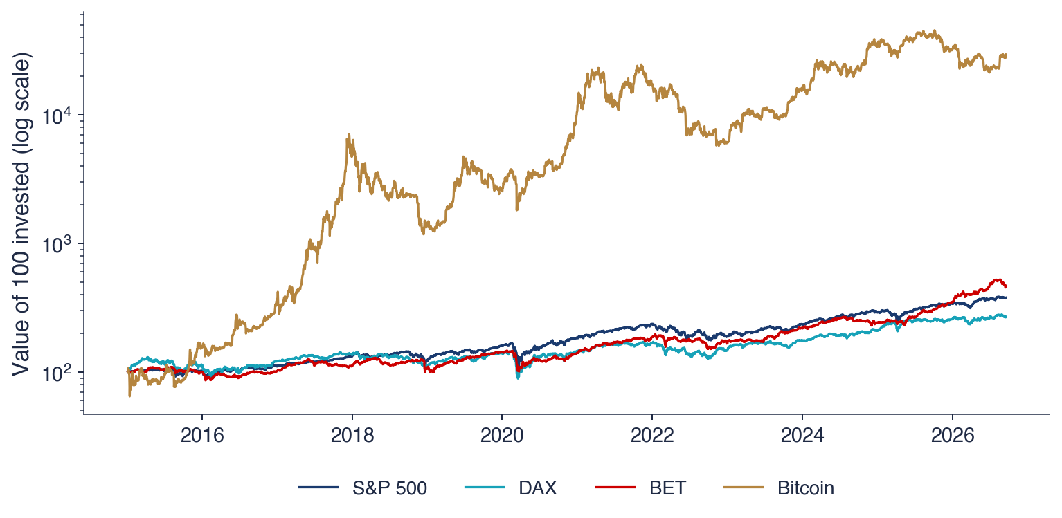

 SFM_ch1_data_quality