Chapter 11: Fractal markets hypothesis and long memory
Daniel Traian PELE
Bucharest University of Economic Studies IDA Institute Digital Assets Blockchain Research Center AI4EFin Artificial Intelligence for Energy Finance Romanian Academy, Institute for Economic Forecasting MSCA Digital Finance
The previous chapters established two facts that seem to pull in opposite directions. Daily returns are almost uncorrelated at small lags, as the weak form of the efficient market hypothesis requires (Chapter 7); their volatility, however, is persistent: turbulent days follow turbulent days (Chapters 8 and 9). This chapter asks the question at the scale of long lags: do today's returns remember what happened months ago? The central tool is the Hurst exponent \(H\), which measures at the same time the memory of a series and the way its risk grows with the horizon. For a random walk, \(H = 0.5\).
The fractal market hypothesis (FMH) of Edgar Peters adds a second theme: who trades, and over which horizon. The market is stable when it contains investors with very different horizons, from minutes to decades, and crises arise when these horizons collapse into one. The hypothesis is stated verbally, but it has statistical consequences that can be tested: the self-similarity of returns across scales, memory over long horizons, and a change of this memory in crises.
On the daily S&P 500 data from 2000 to September 2026, the direction of returns has no long memory: the DFA (detrended fluctuation analysis) exponent of returns is 0.49, inside the 95% band of memoryless series, \([0.46, 0.54]\). The size of returns, however, has strong long memory: the DFA exponent of absolute returns is 0.95. The same contrast appears in all six markets of the chapter, with one partial exception, the BET, whose returns show a weak persistence. The chapter builds the estimators behind these figures, shows how structural breaks and persistent volatility can mimic long memory, and discusses what the results mean for scaling risk with the horizon.
Autocorrelation function of the daily S&P 500 returns (dark blue), of the absolute returns (purple) and of the squared returns (orange), for lags 1–250; the shaded blue area is the 95% band of an i.i.d. series, \(\pm 0.024\).
Learning outcomes
State the fractal market hypothesis and compare it with the efficient market hypothesis and the adaptive markets hypothesis.
Define self-similarity, the Hurst exponent, fractional Brownian motion, fractional Gaussian noise and the ARFIMA(0,\(d\),0) model.
Compute the R/S statistic step by step and estimate \(H\) with R/S, DFA and the GPH regression; apply Lo's modified R/S test.
Assess an estimate against Monte Carlo bands and recognise spurious long memory produced by structural breaks and by volatility clustering.
Distinguish long memory in returns from long memory in volatility on real data, including with rolling estimates.
Explain how \(H\) changes the scaling of risk with the horizon.
Estimators of Long MemoryDFA, the GPH regression, Lo's test, Monte Carlo bands and their application to the S&P 500.
Spurious Long MemoryStructural breaks, the Nile case, volatility clustering and the checks that separate them from genuine long memory.
Long Memory in VolatilityAutocorrelations of absolute returns, six markets, the shuffle test and the FIGARCH and HAR models.
Rolling Hurst ExponentsDFA exponents on 1000-day windows for the S&P 500, the BET and Bitcoin, and their limitations.
Long Memory and RiskScaling VaR with \(h^H\) instead of the square-root-of-time rule.
AI for Scientific DiscoveryAn open question about the Hurst exponent before crises, how AI could help and the checks it needs.
SummaryThe main ideas, the formulas and self-assessment questions.
Efficient Markets and Fractal Markets
The section starts from the efficient market hypothesis and from the facts that its standard model, the random walk with Normal increments, does not explain. It then introduces the fractal market hypothesis, which describes the market through its investors and their horizons, illustrates it with the 1987 crash and shows which of its statistical consequences can be tested. The section ends with a comparison of the efficient market hypothesis, the fractal market hypothesis and the adaptive markets hypothesis.
The efficient market hypothesis (EMH) states that prices reflect the available information (Fama, 1970). In its weak form, studied in Chapter 7, past returns do not help to anticipate future returns. The associated statistical model is the random walk of log prices, with independent increments. In the language of this chapter, the random walk corresponds to the Hurst exponent \(H = 0.5\), and any systematic departure from 0.5 points to some form of long-range dependence.
The random walk with Normal increments, however, leaves several stylised facts unexplained. Returns have heavy tails (Chapters 2, 3 and 5): extreme days are far more frequent than the Normal distribution allows. Volatility comes in clusters, the volatility clustering of Chapters 8 and 9. And crashes such as that of 19 October 1987, discussed below, do not follow from new information of a comparable size.
There is one more question the EMH does not ask: who trades, and over which horizon. The theory treats all investors as a single representative investor who evaluates information correctly. The fractal market hypothesis starts exactly here: it describes the market as a population of investors with different horizons and ties the stability of the market to the diversity of these horizons.
In brief
EMH (efficient market hypothesis, Fama (1970); Chapter 7): prices reflect the available information, so returns cannot be forecast from past returns
the random walk of prices implies independent increments: in this chapter, \(H = 0.5\)
Facts that the random walk with Normal increments does not explain
The fractal market hypothesis was formulated by Peters (1994). Its starting point is that the market consists of investors with many investment horizons, from traders who hold a position for a few minutes to pension funds that invest for decades. The same price event means different things to these investors, and their interaction drives price dynamics.
Peters states the hypothesis in five claims. First: the market is stable when it contains investors with very different horizons, because they provide liquidity to each other. Second: short horizons react mostly to sentiment and technical information, long horizons to fundamental information. Third: if fundamental information becomes doubtful, long-term investors withdraw or start trading short term; the horizons become uniform and the market becomes unstable. Fourth: the price combines short-term technical trading with long-term fundamental valuation. Fifth: an asset unrelated to the economic cycle has no long-term trend, so its dynamics are dominated by short-term trading and liquidity.
The word "fractal" refers to the structure across scales. If the same kind of mechanism acts on every horizon, returns over different horizons should look statistically alike after a suitable rescaling. This property, self-similarity, is the subject of the next section.
In brief
FMH (fractal market hypothesis) Peters (1994): the market is made of investors with many investment horizons, from minutes to decades
The five statements of Peters
the market is stable when it contains investors with many different horizons: this ensures liquidity
short horizons react to sentiment and technical information; long horizons react to fundamental information
if the fundamental information becomes doubtful, long-term investors leave or start to trade short term: horizons become uniform and the market becomes unstable
prices combine short-term technical trading and long-term fundamental valuation
an asset without a link to the economic cycle has no long-term trend: short-term trading and liquidity dominate
The example on the slide makes the mechanism concrete. A stock falls by 3% one morning. For a day trader, whose horizon is a few hours, a 3% fall is a large move that can wipe out the day's gains, and the reaction is to sell. For a pension fund with a ten-year horizon, the same fall is small compared with the variation it expects over that horizon, and the lower price is an opportunity to buy.
The two types of investor are therefore natural counterparties. The long-horizon investor supplies the liquidity the short-horizon investor needs, and the price adjusts in an orderly way, without jumps. In this interpretation, liquidity is not a property of the asset but the result of participants valuing the same price over different horizons.
If the pension fund also starts to judge the market over the next few hours, for instance because it no longer trusts fundamental information, nobody buys. Liquidity disappears and the fall accelerates. The same pattern of behaviour can repeat on every horizon, which gives returns that are statistically alike at different scales: the meaning of "fractal" in the name of the hypothesis.
In brief
A share falls by 3% in one morning
a day trader (horizon: hours) sees a large move and sells
a pension fund (horizon: ten years) sees a small move relative to its horizon and buys at a lower price
The long-horizon investor supplies the liquidity that the short-horizon investor demands: the price stays orderly
If the pension fund also starts to fear the next hours, nobody buys: there is no liquidity and the fall accelerates
Fractal: the same pattern of behaviour repeats at every horizon, with statistically similar returns at different scales
On 19 October 1987, the S&P 500 fell by about 20% in a single day (Carlson, 2007). The chart published by the Federal Reserve shows the index in the days around the crash: the fall happened in a single session, without new economic information of a comparable size.
The FMH interpretation focuses on horizons. Portfolio insurance and automated trading programmed to sell when prices fall made long-horizon portfolios sell exactly like short-term traders. All horizons effectively collapsed into one, and the buyers who should have provided liquidity disappeared.
A testable consequence follows from this interpretation. If short horizons dominate in crises, the statistical structure of returns across scales should change during crisis periods. The next slide shows how this idea translates into quantities that can be estimated.
In brief
19 October 1987: the S&P 500 fell by about 20% in one day Carlson (2007)
The FMH reading
portfolio insurance and program trading made long-term portfolios sell like short-term traders
all horizons became one horizon: buyers disappeared
Testable consequence: in crises, short horizons dominate and the statistical structure across scales changes
The FMH is a verbal theory, without a probabilistic model of its own. Its statistical consequences can still be tested, and the chapter follows three of them. The first is self-similarity: the distribution of \(h\)-day returns should look the same after rescaling by \(h^H\) (Section 2). The second is memory: the Hurst exponent \(H\) measures dependence over long horizons (Sections 3–5). The third is change: in crises, \(H\) and the weight of short horizons should shift (Section 8).
The reference studies for the third consequence are those of Kristoufek (2012) and Kristoufek (2013) on the 2008 financial crisis. The first uses local Hurst exponents, estimated on rolling windows, and the second uses wavelet power, which shows how the variance of a series is distributed across time scales and how this distribution changes over time. Both studies analyse major stock indices.
Their result agrees with the FMH: the most turbulent periods of the crisis coincide with the dominance of short investment horizons. The result does not prove Peters's mechanism, but it shows that his prediction about horizons has a measurable counterpart in the data.
In brief
The FMH is a verbal theory; its statistical consequences can be tested
self-similarity: the distribution of \(h\)-day returns looks the same after rescaling by \(h^H\) (Section 2)
memory: the Hurst exponent \(H\) measures dependence over long horizons (Sections 3–5)
change: in crises, \(H\) and the share of short horizons should change (Section 8)
The table compares three hypotheses about markets. The EMH (Fama, 1970) works with a representative investor, and prices are always right given the available information. The FMH (Peters, 1994) works with investors on many horizons, and stability comes from their diversity. The adaptive markets hypothesis (AMH) of Lo (2004) describes the market as an ecosystem of "species" of investors and strategies that compete and adapt, so that the degree of efficiency changes with the environment.
The row on memory translates the three hypotheses into the language of the chapter. For the EMH, \(H = 0.5\). For the FMH, \(H\) may differ from 0.5, because the structure of horizons can produce long-range dependence. For the AMH, \(H\) varies over time with market conditions. The last row shows how each hypothesis sees crises: for the EMH they lie outside the theory, for the FMH they are collapses of horizons, and for the AMH they are episodes in which many strategies die out at the same time.
The three hypotheses are not rival tests among which the data would pick one. The EMH is a good approximation in normal conditions; the FMH and the AMH try to explain where and why this approximation breaks down. For statistical analysis, the practical consequence is that \(H\) must be estimated both on the full sample and on subperiods.
The three are not rival tests: the FMH and the AMH explain when and why the EMH approximation fails
Section summary
The EMH treats the market as a single representative investor and implies \(H = 0.5\). The FMH describes the market through investors with different horizons, ties stability to the diversity of these horizons and interprets crashes such as that of 1987 as their collapse. Its testable consequences are self-similarity, memory over long horizons and a change of this memory in crises. The next section defines the first of them, self-similarity.
Self-Similarity and Fractals
The section introduces the geometric language of the chapter. It starts from the work of Benoît Mandelbrot, defines fractal dimension and self-similar processes, and shows that self-similarity has a direct consequence for returns: the standard deviation of \(h\)-day returns grows like \(h^H\). The slope of this growth, estimated for the S&P 500, the BET and Bitcoin, gives a first estimate of the Hurst exponent.
Benoît Mandelbrot and the Measurement of Roughness
Benoît Mandelbrot (1924–2010) brought to finance the idea that roughness can be measured. In Mandelbrot (1963) he showed that changes in cotton prices have heavy tails and that their distribution looks alike at the daily, monthly and yearly scale. The model he proposed then was the family of \(\alpha\)-stable distributions, the subject of Chapter 3, which are invariant, up to a rescaling, under the summation of independent variables.
In Mandelbrot (1967), Mandelbrot asked a question of geometry: how long is the coast of Britain? The measured length of a coastline grows as the ruler gets shorter, because a shorter ruler follows more of its bays and headlands. The rate at which the length grows as the ruler shrinks defines a fractal dimension, which measures how rough the curve is.
Mandelbrot & Van Ness (1968) defined fractional Brownian motion, the central probabilistic model of this chapter. The common idea of these papers is the notion of a fractal: an object whose parts resemble the whole, either exactly, as in geometric figures, or in distribution, as in price series. The Mandelbrot set in the picture is the best-known visual example.
In brief
Mandelbrot (1963): cotton prices have heavy tails and look alike at daily, monthly and yearly scales
The simplest fractal dimension is the similarity dimension. If an object consists of \(N\) copies of itself, each scaled down by the factor \(1/s\), its dimension is \(D = \ln N / \ln s\). The definition reproduces the usual dimensions: a segment consists of 2 halves, so \(D = \ln 2/\ln 2 = 1\); a square consists of 4 squares with half the side, so \(D = \ln 4/\ln 2 = 2\).
For fractal objects the dimension is not an integer. The Koch curve consists of 4 copies of itself, each scaled down by 3, so \(D = \ln 4/\ln 3 = 1.262\): more than a line, less than a surface. The Sierpinski triangle consists of 3 copies scaled down by 2, with \(D = \ln 3/\ln 2 = 1.585\). For the west coast of Britain, Mandelbrot (1967) gives \(D \approx 1.25\).
The link with finance runs through the graph of a price path. For fractional Brownian motion, the fractal dimension of the graph is \(D = 2 - H\). An ordinary Brownian motion, with \(H = 0.5\), has \(D = 1.5\). A path with persistent trends (\(H > 0.5\)) is smoother and has \(D < 1.5\); a path with frequent reversals (\(H < 0.5\)) is rougher and has \(D > 1.5\).
In brief
Similarity dimension: an object made of \(N\) copies of itself, each scaled by \(1/s\), has \(D = \ln N/\ln s\)
a segment: 2 halves, \(D = \ln 2/\ln 2 = 1\); a square: 4 quarters of side \(1/2\), \(D = \ln 4/\ln 2 = 2\)
the Koch curve: 4 copies scaled by \(1/3\), \(D = \ln 4/\ln 3 = 1.262\)
the Sierpinski triangle: 3 copies scaled by \(1/2\), \(D = \ln 3/\ln 2 = 1.585\)
A stochastic process \(X_t\) is self-similar with exponent \(H\) if, for every \(c > 0\),
\[X_{ct} \overset{d}{=} c^H X_t,\]
(11.1)
where \(\overset{d}{=}\) denotes equality in distribution (Franke, Härdle & Hafner (2019), Def. 14.1). Stretching the time axis by the factor \(c\) has the same effect as stretching the values by the factor \(c^H\). The exponent \(H\) is called the Hurst exponent.
The Brownian motion of Chapter 4 is self-similar with \(H = 1/2\):\(W_{ct} \overset{d}{=} \sqrt{c}\,W_t\). For log prices with self-similar increments, (11.1) has a direct consequence for multi-day returns. If \(r_t^{(h)}\) is the \(h\)-day return, its standard deviation is \(\mathrm{sd}(r_t^{(h)}) = h^H\,\mathrm{sd}(r_t)\). The square-root-of-time rule, \(\sqrt{h}\), routinely used to scale volatility and VaR, is the special case \(H = 1/2\).
The relation gives a first estimator of \(H\). Taking logarithms, \(\ln \mathrm{sd}(r^{(h)}) = \ln \mathrm{sd}(r) + H \ln h\), so on a chart with both axes logarithmic the points must lie on a line with slope \(H\). The next slide applies this estimator to three markets.
In brief
Self-similar processFranke, Härdle & Hafner (2019), Def. 14.1: \(X_{ct} \overset{d}{=} c^H X_t\) for every \(c > 0\); \(H\) is the Hurst exponent
\(\overset{d}{=}\): equal in distribution; stretching time by \(c\) equals stretching values by \(c^H\)
Brownian motion (Chapter 4) is self-similar with \(H = 1/2\): \(W_{ct} \overset{d}{=} \sqrt{c}\,W_t\)
Consequence for log prices with self-similar increments
\(\mathrm{sd}(r_t^{(h)}) = h^H\,\mathrm{sd}(r_t)\), where \(r_t^{(h)}\) is the \(h\)-day return and sd the standard deviation
the square-root-of-time rule \(\sqrt{h}\) is the special case \(H = 1/2\)
A first estimator of \(H\): the slope of \(\ln \mathrm{sd}(r^{(h)})\) on \(\ln h\)
Question for the room We count boxes on the fBm path with H = 0.5 (extra computation, not in the lecture). Which dimension comes out?
Answer
About 1.5: the slope is 1.47 with ε from 1/2 to 1/128, close to D = 2 − H = 1.5. The path is a curve, but so rough that the number of boxes grows like ε^(−1.5), not like ε^(−1). For H = 0.1 the count gives only 1.74 instead of 1.9: with 1000 points the roughness below the time step is invisible, so D is underestimated for very rough paths.
Question for the room S&P 500: is the ratio of the 10-day to the daily standard deviation of returns above or below √10 = 3.16?
Answer
Below: 2.80. The daily S&P 500 returns have a negative first-order autocorrelation, −0.099, so consecutive days partly offset each other (mild mean reversion). The BET has 3.50, above √10 (positive autocorrelation), and Bitcoin 3.20, close to √10.
The chart shows, for the S&P 500, the BET and Bitcoin, the standard deviation of \(h\)-day returns divided by the standard deviation of daily returns, for horizons from one day to 250 days, with the data available up to 18 September 2026. The \(h\)-day returns are computed on non-overlapping blocks. Both axes are logarithmic, and the dashed line is the square-root-of-time rule, with slope 0.5.
The estimated slopes are 0.48 for the S&P 500, 0.59 for the BET and 0.55 for Bitcoin. The S&P 500 curve lies below the dashed line at every horizon: multi-day risk grows somewhat more slowly than the \(\sqrt{h}\) rule predicts. The BET curve lies above the line, and the gap widens with the horizon: the one-year risk is larger than the daily risk scaled by \(\sqrt{250}\). The Bitcoin curve is close to the line at short horizons and above it at long horizons.
The slope summarises all horizons from 1 to 250 days, and the points at long horizons, where the BET departs most, have a large influence on it. The next slide reads the chart at a single horizon, 10 days, and links the departures from \(\sqrt{h}\) to the autocorrelations of daily returns.
In brief
Standard deviation of non-overlapping \(h\)-day returns divided by the daily one, \(h = 1, \dots, 250\), log scales; data to 18 September 2026
Slopes: S&P 500 \(0.48\), BET \(0.59\), Bitcoin \(0.55\); the square-root rule has slope 0.5
For the S&P 500, the standard deviation of 10-day returns is 2.80 times the daily standard deviation, below the value \(\sqrt{10} = 3.16\) of the square-root rule. The explanation is a slight mean reversion: the first-order autocorrelation of daily returns is negative, \(-0.099\). When consecutive returns tend to offset each other partly, the variance of their sum is smaller than the sum of their variances.
For the BET, the 10-day ratio is 3.50, above \(\sqrt{10}\), which points to positive autocorrelation. One source of it is the thin trading of the index's early years, discussed in Chapter 7: when some stocks in the index do not trade every day, new information enters the price with a delay, and the index adjusts slowly, over several consecutive days with the same sign. For Bitcoin, the ratio is 3.20, close to \(\sqrt{10}\).
The slopes must be read with caution. At the 250-day horizon there are only a few dozen non-overlapping blocks, and a standard deviation estimated from so few values is imprecise. A slope of 0.55 cannot be told apart from 0.5 without a confidence band. The chapter therefore builds better estimators of \(H\) and Monte Carlo bands for them.
In brief
S&P 500: 10-day risk is \(2.80\) times the daily risk, below \(\sqrt{10} = 3.16\)
slight mean reversion: daily returns have a negative first-order autocorrelation, \(-0.099\)
thin trading in the early years makes the index adjust slowly (Chapter 7)
Bitcoin: \(3.20\) times, close to \(\sqrt{10}\)
Caution: there are only a few dozen non-overlapping 250-day blocks; the slope is imprecise, so it needs a proper estimator and a band
Section summary
A self-similar process keeps its distribution when time is stretched by \(c\) and values by \(c^H\); for returns, the consequence is that the \(h\)-day standard deviation grows like \(h^H\). The scaling slopes are 0.48 for the S&P 500, 0.59 for the BET and 0.55 for Bitcoin, against 0.5 for the square-root-of-time rule, but they rest on few blocks at long horizons. The next section introduces an estimator of \(H\) with a longer history, Hurst's R/S statistic.
Hurst, the Nile and the R/S Statistic
The Hurst exponent is named after a hydrologist who designed reservoirs on the Nile. The section shows how the problem of reservoir capacity led to the R/S statistic, computes the statistic step by step on a small example, builds an estimator of \(H\) from it, and shows that in small samples this estimator is biased upwards even for data without memory.
Harold Edwin Hurst (1880–1978) was a British hydrologist who worked in Egypt from 1906 and designed reservoirs on the Nile. His practical question was how large a reservoir must be to release the mean flow of the river every year. A reservoir that receives a year's flow and releases the mean fills up in high-flow years and empties in low-flow years, so the capacity needed equals the range of the cumulative deviations of the flows from their mean.
Hurst (1951) studied how this range grows with the number of years \(n\). For independent flows, theory predicts growth like \(n^{0.5}\). In series of river flows, rainfall and tree-ring thickness, Hurst found growth like \(n^K\), with \(K\) averaging about 0.73. The difference between the exponents is amplified over long periods: the required capacity grows much faster with the number of years than the assumption of independent flows predicts.
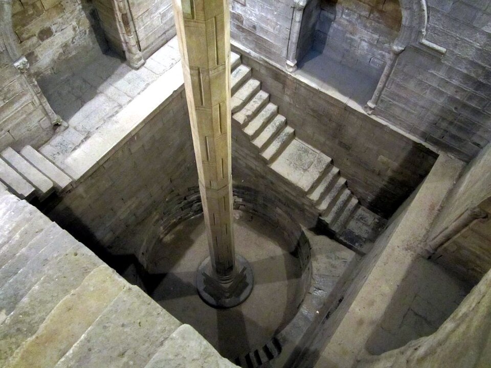
The explanation is that high-flow years tend to follow high-flow years, and dry years follow dry years. Deviations from the mean do not offset each other quickly but accumulate over long periods. This is long memory, and Hurst's exponent became its standard measure. The Nilometer on Roda Island in Cairo, in the picture, built in 861, is one of the historical sources of data on the level of the Nile.
In brief
Hurst (1880–1978), a British hydrologist who worked in Egypt from 1906, designed reservoirs on the Nile
the capacity needed to deliver the average flow every year equals the range of the cumulative deviations of the inflows from their mean
Hurst (1951): for independent inflows this range grows like \(n^{0.5}\); in river flows, rainfall and tree rings it grows like \(n^{K}\) with \(K\) about \(0.73\) on average
years of high flow follow years of high flow: long memory
The R/S statistic formalises Hurst's calculation for a block of observations \(x_1, \dots, x_n\) with mean \(\bar x\). The cumulative deviations from the mean are \(Y_k = \sum_{j=1}^{k} (x_j - \bar x)\), for \(k = 1, \dots, n\); by construction, \(Y_n = 0\). Their range is \(R_n = \max_k Y_k - \min_k Y_k\), and the standard deviation of the block is \(S_n = \sqrt{\frac1n \sum_j (x_j - \bar x)^2}\). The rescaled range statistic, defined in Franke, Härdle & Hafner (2019), 14.4.1, is
\[(R/S)_n = \frac{R_n}{S_n}\]
(11.2)
Dividing by \(S_n\) removes the unit of measurement, so \((R/S)_n\) is comparable across assets with different volatilities.
What matters is how \((R/S)_n\) behaves as \(n\) grows. For i.i.d. data with finite variance, \((R/S)_n\) grows like \(n^{1/2}\), as a consequence of the functional central limit theorem: the cumulative deviations behave like a Brownian bridge, whose range is of order \(\sqrt{n}\). Under long memory, the cumulative deviations wander further from zero, and \((R/S)_n\) grows like \(n^H\), with \(H > 1/2\).
A useful property of the statistic is its robustness to heavy tails (Mandelbrot & Wallis, 1969). An extreme value inflates both the range \(R_n\) and the standard deviation \(S_n\), and their ratio is affected much less than either of them. For financial returns, with their heavy tails, this property is an advantage over estimators built directly on variances.
In brief
Block \(x_1, \dots, x_n\) with mean \(\bar x\); cumulative deviations\(Y_k = \sum_{j=1}^{k}(x_j - \bar x)\), \(k = 1, \dots, n\)
\[\log_{10}(R/S)_n = \log_{10} c + H \log_{10} n + e_n, \qquad \hat H = \frac{\sum (u - \bar u)(v - \bar v)}{\sum (u - \bar u)^2}\]
Question for the room The OLS slope of log₁₀ (R/S)_n for the S&P 500 returns is 0.530. What does it become for the absolute returns |r|?
Answer
About 0.86 (0.861), far above the i.i.d. band [0.51, 0.57]: long memory in volatility. For the returns, 0.530 lies inside the band, because R/S is biased upwards in small samples.
Question for the room ▶ moves to 8-day windows of the S&P 500. On 9–18 March 2020 the standard deviation is 7.56%, about 15 times that of the lecture example (0.489). How does (R/S)₈ compare with 1.788?
Answer
It is of the same order: 1.530. R and S grow together with volatility, so the ratio has no unit; for 8 values R/S stays between about 1.5 and 2.8 (2.317 in January 2000, 2.774 in October 2008, 2.155 in September 2026). Dividing by S makes the statistic comparable across assets.
The example applies the definition to eight daily returns, in per cent: 0.5; −0.3; 0.8; −0.2; 0.6; −0.1; 0.4; −0.7. Their sum is 1.0, so the mean is \(\bar x = 0.125\). The deviations from the mean are +0.375; −0.425; +0.675; −0.325; +0.475; −0.225; +0.275; −0.825, and their running sums give \(Y_1, \dots, Y_8\): 0.375; −0.050; 0.625; 0.300; 0.775; 0.550; 0.825; 0.000.
The chart shows the deviations as bars and the cumulative deviations as a line. The maximum of the cumulative deviations is 0.825, reached at \(k = 7\), and the minimum is −0.050, at \(k = 2\), so the range is \(R = 0.825 - (-0.050) = 0.875\). The sum of squared deviations is 1.915, so \(S = \sqrt{1.915/8} = 0.489\). The R/S statistic of the block is \((R/S)_8 = 0.875/0.489 = 1.788\).
The last value, \(Y_8 = 0\), checks the computation: the deviations from the mean always sum to zero. A single block, however, gives a single point, and the exponent \(H\) describes how \((R/S)_n\) changes with the block size. Estimating it requires many block sizes, which is what the procedure on the next slide does.
The standard procedure for estimating \(H\) with R/S follows Mandelbrot & Wallis (1969). For a series of \(N\) returns, block sizes \(n\) are chosen between 10 and \(N/4\), equally spaced on a logarithmic scale. For each \(n\), the series is split into \(\lfloor N/n \rfloor\) non-overlapping blocks, R/S is computed in each block, and the average of these values is \((R/S)_n\).
The exponent is then estimated by ordinary least squares (OLS) in the regression
\[\ln (R/S)_n = \ln c + H \ln n + e_n,\]
(11.3)
where \(c\) is a constant and \(e_n\) is the regression error. The estimated slope \(\hat H\) is the R/S estimator of the Hurst exponent. The lower limit of 10 observations avoids blocks so small that R/S is dominated by sampling effects, and the upper limit \(N/4\) guarantees at least four blocks for each average.
The log-log plot of \((R/S)_n\) against \(n\) is the main diagnostic tool. If the points lie on a line, a single scaling exponent describes the series; a curvature or a change of slope points to different behaviour on short and long scales. The method is applied to returns, which are stationary, not to prices: for a price series, the cumulative deviations grow linearly with the block size, and \((R/S)_n\) grows roughly like \(n\), whatever the memory.
The table summarises the three regimes of \(H\). For \(0 < H < 0.5\), increments are negatively correlated and memory is anti-persistent: a rise tends to be followed by a fall. The path is rough, with fractal dimension \(D = 2 - H > 1.5\). For \(H = 0.5\), increments are uncorrelated, as in a random walk, and \(D = 1.5\). For \(0.5 < H < 1\), increments are positively correlated, memory is persistent and produces trends, and the path is smoother, with \(D < 1.5\).
A common confusion is to read \(H\) as a probability. \(H = 0.7\) does not mean that the sign of the return repeats on 70% of days. \(H\) is a scaling exponent: it describes how the variability of sums grows with the length of the period and, equivalently, how slowly autocorrelations decay at long lags.
Mandelbrot & Wallis (1968) gave biblical names to the two departures from the independent Gaussian model. The Noah effect refers to extreme values: heavy tails, the flood. The Joseph effect refers to long runs of high or low values, as in "seven years of plenty, seven years of famine". The two effects are distinct and have different measures: \(H\) measures the Joseph effect, and the tail index of Chapter 5 measures the Noah effect.
In brief
\(H\)
increments
memory
path (\(D = 2 - H\))
\(0 < H < 0.5\)
negatively correlated
anti-persistent: reversals
rough, \(D > 1.5\)
\(H = 0.5\)
uncorrelated
none (random walk)
\(D = 1.5\)
\(0.5 < H < 1\)
positively correlated
persistent: trends
smoother, \(D < 1.5\)
\(H\) is not a probability: \(H = 0.7\) does not mean “70% chance that the sign repeats”
The result that \((R/S)_n\) grows like \(n^{1/2}\) for i.i.d. data is asymptotic. Anis & Lloyd (1976) computed the exact expected value of \((R/S)_n\) for independent Normal summands and showed that it approaches \(c\,n^{1/2}\) only for large \(n\); for small \(n\),\((R/S)_n\) grows faster than \(n^{1/2}\). The slope estimated on blocks from \(n = 10\) to \(N/4\) is therefore above 0.5 even for data without any memory.
A Monte Carlo simulation with 500 i.i.d. Normal series measures this bias. The mean of the R/S estimator is 0.588 for series of 250 observations, 0.562 for 1000 observations and 0.547 for 5000 observations. The bias shrinks with the length of the series but does not vanish at the usual lengths of financial data. For \(N = 1000\), 95% of the estimates lie in the interval \([0.50, 0.63]\).
The practical rule is to compare \(\hat H\) not with 0.5 but with the distribution of \(\hat H\) under the null hypothesis, simulated for the same \(N\) and with the same block sizes. An R/S estimate of 0.56 on 1000 observations is no evidence of long memory: it is exactly the mean of the estimator for memoryless data. Section 5 builds such bands for all the estimators of the chapter.
In brief
For i.i.d. data, \((R/S)_n\) approaches \(c\,n^{1/2}\) only for large \(n\); for small \(n\) it grows faster Anis & Lloyd (1976)
the fitted slope over \(n = 10, \dots, N/4\) is above 0.5 even without any memory
Monte Carlo, 500 i.i.d. Normal series
mean \(\hat H_{R/S}\): \(0.588\) for \(N = 250\), \(0.562\) for \(N = 1000\), \(0.547\) for \(N = 5000\)
95% band for \(N = 1000\): \([0.50, 0.63]\)
Rule: compare \(\hat H\) with the distribution of \(\hat H\) under the null hypothesis for the same \(N\), not with 0.5 (Section 5)
Section summary
Hurst's R/S statistic measures the range of the cumulative deviations relative to the standard deviation, and its slope on a log-log plot estimates \(H\). For independent data the slope is 0.5 asymptotically, but in usual samples it is biased upwards: on average 0.562 for 1000 i.i.d. observations. \(H\) measures the Joseph effect, persistence, not the Noah effect, extreme values. The next section gives the exact definition of long memory and the models that generate it.
Long Memory: Definitions and Models
The section defines long memory through autocorrelations and through the spectral density and compares it with the short memory of ARMA models. It then introduces two families of long-memory models: fractional Brownian motion, together with its increments, fractional Gaussian noise, and the ARFIMA model, built by fractional differencing. For each model, the slides compute the autocorrelations and show simulated paths.
Let \(X_t\) be a stationary process with autocorrelation function (ACF) \(\rho(k)\). The process has long memory if its autocorrelations are not summable, \(\sum_k |\rho(k)| = \infty\)(Franke, Härdle & Hafner (2019), 14.1). The usual parametric form of this property is hyperbolic decay,
\[\rho(k) \sim C\,k^{2d - 1}, \qquad k \to \infty,\]
(11.4)
with a constant \(C > 0\) and the memory parameter \(0 < d < 0.5\); the symbol \(\sim\) means that the ratio of the two sides tends to 1. For \(0 < d < 0.5\) the exponent \(2d - 1\) lies between −1 and 0, so the sum of the autocorrelations diverges. Hyperbolic decay implies non-summability; the converse does not hold in general, but all the models of this chapter have the form (11.4).
In the frequency domain, the same property appears as a pole of the spectral density at zero: \(f(\lambda) \sim C\,\lambda^{-2d}\) as \(\lambda \to 0\). The spectral density \(f(\lambda)\) decomposes the variance of the series over frequencies, and frequencies close to zero correspond to very long cycles. A long-memory series has a large share of its variance in these long cycles.
Short memory is that of ARMA (autoregressive moving average) models. For an AR(1) with coefficient \(\phi\),\(\rho(k) = \phi^k\) decays exponentially, and the sum \(\sum_k |\phi|^k\) is finite, equal to \(1/(1 - |\phi|)\). The difference between \(\phi^k\) and \(k^{2d-1}\) is the difference between a shock forgotten after a few periods and a shock that still matters after hundreds of periods. The link with the Hurst exponent is \(d = H - 1/2\).
In brief
Stationary \(X_t\) with autocorrelations \(\rho(k)\) (ACF, autocorrelation function); long memoryFranke, Härdle & Hafner (2019), 14.1:
\(\sum_{k} |\rho(k)| = \infty\): the autocorrelations are not summable
the usual form: hyperbolic decay \(\rho(k) \sim C\,k^{2d - 1}\) as \(k \to \infty\), with the memory parameter\(0 < d < 0.5\); it implies non-summability, the converse does not hold in general
in frequency: the spectral density has a pole at zero, \(f(\lambda) \sim C\,\lambda^{-2d}\) as \(\lambda \to 0\)
\(C > 0\): a constant; \(\sim\): the ratio of the two sides tends to 1; \(f(\lambda)\): the share of variance at frequency \(\lambda\) (long cycles: \(\lambda\) near 0)
Short memory: ARMA (autoregressive moving average) models, e.g. AR(1) with \(\rho(k) = \phi^k\)
The example compares two processes with the same first-order autocorrelation. The first is a fractional Gaussian noise with \(H = 0.8\), the long-memory model defined a few slides further on. Its first-order autocorrelation is \(\rho(1) = 2^{2H-1} - 1 = 2^{0.6} - 1 = 0.516\), and at long lags the autocorrelations are \(\rho(10) = 0.191\),\(\rho(50) = 0.100\) and \(\rho(100) = 0.076\).
The second process is an AR(1) with \(\phi = 0.516\), chosen to have the same first-order autocorrelation. Its autocorrelations are the powers of \(\phi\):\(\rho(10) = 0.516^{10} = 0.0013\), and \(\rho(100) = 0.516^{100}\) is practically zero.
In the short run, the two processes cannot be told apart by their first autocorrelation. In the long run, they are very different: after 10 lags, the autocorrelation of the long-memory process is two orders of magnitude larger than that of the AR(1), and after 100 lags a shock still matters only for the long-memory process. An ARMA model fitted to the autocorrelations at small lags cannot reproduce such persistence.
In brief
Long memory: fractional Gaussian noise (next slides) with \(H = 0.8\)
Fractional Brownian motion (fBm) \(B_H(t)\), with \(0 < H < 1\), is the Gaussian process with continuous paths that is self-similar with exponent \(H\) and has stationary increments (Mandelbrot & Van Ness, 1968), with the properties given in Franke, Härdle & Hafner (2019), Def. 14.2. These three properties determine it up to a scale constant: it is the natural generalisation of Brownian motion to Hurst exponents other than 1/2.
The moments of the process are given by Theorem 14.1 of Franke, Härdle & Hafner (2019). The process starts at zero, \(B_H(0) = 0\), has mean zero and variance \(E[B_H(t)^2] = \sigma^2 |t|^{2H}\), where \(\sigma^2\) is the variance at \(t = 1\). The covariance between two points in time is
A variance growing like \(|t|^{2H}\) is the self-similarity (11.1) expressed through moments.
For \(H = 1/2\), formula (11.5) becomes \(\sigma^2 \min(t, s)\), the covariance of Brownian motion, whose increments are independent. For \(H \neq 1/2\), increments over disjoint intervals are correlated at all lags: positively for \(H > 1/2\), negatively for \(H < 1/2\). Because the process is Gaussian and its covariance is known exactly, it can be simulated exactly from the covariance matrix of the increments; the circulant embedding method makes this computation fast even for long series.
In brief
Fractional Brownian motion (fBm) \(B_H(t)\), \(0 < H < 1\)Mandelbrot & Van Ness (1968); Franke, Härdle & Hafner (2019), Def. 14.2: a Gaussian process with continuous paths, self-similar with exponent \(H\) and with stationary increments
Question for the room ▶ raises H of the fGn from 0.55 to 0.95. How does ρ(100) change?
Answer
It rises from about 0.001 (H = 0.55) to about 0.54 (H = 0.95); at H = 0.8 it is 0.076. For large H, ρ(k) decays like k^(2H − 2), that is very slowly. An AR(1) with the same ρ(1) has ρ(100) practically 0 for every H: its decay is geometric.
Question for the room What is the first-order autocorrelation of the increments of the path with H = 0.7?
Answer
In theory 2^(2H − 1) − 1 = 2^0.4 − 1 = 0.32; on the 1000 simulated increments, 0.32 (0.316). For H = 0.3: −0.23 in the data, −0.24 in theory. H is neither an autocorrelation nor a probability.
The left panel shows three fBm paths of 1000 steps, with \(H = 0.3\),\(0.5\) and \(0.7\), simulated from the same random numbers. Using the same random numbers means that the differences between the paths come only from the exponent. The right panel shows the first 150 increments of each path, that is, the corresponding fractional Gaussian noise.
The path with \(H = 0.7\) makes long excursions in one direction and reaches the largest amplitude, more than 75 units below its starting point. The path with \(H = 0.3\) changes direction often and stays close to zero. Brownian motion, with \(H = 0.5\), lies in between. The difference in amplitude follows directly from the variance \(\sigma^2 t^{2H}\): after 1000 steps, \(t^{2H}\) is much larger for \(H = 0.7\) than for \(H = 0.3\).
The increments on the right look almost the same for the three exponents: memory is not visible to the naked eye in the series of increments but in their accumulation. It does show up in the autocorrelations. The first-order autocorrelation of the simulated increments is 0.32 for \(H = 0.7\) and −0.23 for \(H = 0.3\), close to the theoretical values 0.32 and −0.24.
In brief
The same random numbers, \(H = 0.3\), \(0.5\), \(0.7\) (as in SFEfbmplot); right: the first 150 increments
\(H = 0.7\): long excursions and a wide range; \(H = 0.3\): frequent reversals, a narrow range; lag-1 autocorrelation of the increments \(0.32\) and \(-0.23\) (theory \(0.32\) and \(-0.24\))
Fractional Gaussian noise (fGn) is the series of fBm increments, \(Y_k = B_H(k+1) - B_H(k)\)(Franke, Härdle & Hafner (2019), 14.3). Because fBm has stationary increments, fGn is a stationary series, the counterpart of white noise with memory. Its autocorrelation function follows from (11.5):
and for large \(k\),\(\rho(k) \approx H(2H - 1)\,k^{2H-2}\). Comparing with (11.4), the exponent \(2H - 2\) equals \(2d - 1\) for \(d = H - 1/2\).
The sign of the factor \(H(2H - 1)\) gives the three regimes. For \(1/2 < H < 1\), all autocorrelations are positive and not summable: long memory, with \(d = H - 1/2\) between 0 and 1/2. For \(H = 1/2\), all autocorrelations from lag 1 on are zero: white noise. For \(0 < H < 1/2\), the autocorrelations are negative and summable: anti-persistence, a form of memory different from long memory in the sense of definition (11.4).
fGn is the model behind the R/S and DFA estimators. For an fGn series, both estimators estimate the Hurst exponent \(H\) of the fBm the series comes from. This is why returns are treated as a possible fGn and log prices as a possible fBm.
In brief
Fractional Gaussian noise (fGn): the increments \(Y_k = B_H(k + 1) - B_H(k)\), a stationary series Franke, Härdle & Hafner (2019), 14.3
Question for the room On the slide, the sample ACF of the fGn with H = 0.8 lies below the theoretical one. Why?
Answer
Estimating the mean removes part of the slow component of the series: with long memory the sample mean follows the long waves, and the deviations from it are less correlated. Over lags 1–50 the sample ACF is on average 0.040 below the theoretical one. The circulant-embedding simulation is exact, and the fGn ACF formula is exact at every lag.
The left panel shows the sample ACF of two simulated fGn series of 5000 values, together with the theoretical ACF given by (11.6). For \(H = 0.8\), the autocorrelations start at \(\rho(1) = 0.516\) and decay slowly, remaining clearly positive at lag 50. For \(H = 0.2\), the first-order autocorrelation is \(\rho(1) = -0.340\), and those at larger lags are almost zero.
The right panel has both axes logarithmic. On these axes, the hyperbolic decay \(k^{2H-2}\) of the fGn with \(H = 0.8\) is a straight line, which reaches about 0.03 at lag 1000. The curve of the AR(1) with the same \(\rho(1) = 0.516\) plunges below \(10^{-4}\) before lag 15. The chart makes the difference between long and short memory visible: a power law against an exponential.
In the left panel, the sample points for \(H = 0.8\) lie systematically below the theoretical curve. The phenomenon is typical of long-memory series. The sample ACF is computed around the sample mean, and in a long-memory series the sample mean partly follows the long cycles of the series; subtracting it removes part of the slow component and shrinks the estimated autocorrelations.
In brief
Left: sample and theoretical ACF for \(H = 0.8\) and \(H = 0.2\) (as in SFEfgnacf); \(\rho(1) = 0.516\) and \(-0.340\)
Right, log scales: hyperbolic decay (a straight line) against the exponential decay of an AR(1) with the same \(\rho(1)\)
The sample ACF of a long-memory series lies below the theoretical one: estimating the mean removes part of the slow component
The second long-memory model comes from time-series econometrics (Granger & Joyeux, 1980; Hosking, 1981). The ARFIMA(0,\(d\),0) model (autoregressive fractionally integrated moving average) is defined by
\[(1 - L)^d X_t = \varepsilon_t,\]
(11.7)
where \(\varepsilon_t\) is i.i.d. with mean 0 and variance \(\sigma^2\), and \(L\) is the lag operator, \(L X_t = X_{t-1}\). For \(d = 0\) the model is white noise, and for \(d = 1\) it is the random walk of Chapter 7. What is new is that \(d\) may take non-integer values.
The operator \((1 - L)^d\) with non-integer \(d\) is defined by the binomial expansion (Franke, Härdle & Hafner (2019), 14.2): \((1 - L)^d = \sum_{j \ge 0} \pi_j L^j\), with \(\pi_0 = 1\) and \(\pi_j = \pi_{j-1}(j - 1 - d)/j\). The model can then be written as \(X_t = \varepsilon_t - \sum_{j \ge 1} \pi_j X_{t-j}\): the current value depends on the whole past, with weights that decay slowly, like a power of \(j\). In infinite moving-average form, \(X_t = \sum_{j \ge 0} \psi_j \varepsilon_{t-j}\), with \(\psi_0 = 1\) and \(\psi_j = \psi_{j-1}(j - 1 + d)/j\), each past shock contributes with a weight that also decays like a power.
The autocorrelations have a closed form, \(\rho(k) = \Gamma(1-d)\Gamma(k+d)/[\Gamma(d)\Gamma(k+1-d)]\), where \(\Gamma\) is the gamma function, with \(\Gamma(n) = (n-1)!\) for integers. More useful for computation is the recursion \(\rho(k) = \rho(k-1)(k - 1 + d)/(k - d)\), starting from \(\rho(1) = d/(1 - d)\). For large \(k\),\(\rho(k) \sim C k^{2d - 1}\), so the model has long memory for \(0 < d < 1/2\), with the same parameter \(d\) as in definition (11.4).
The table, taken from Franke, Härdle & Hafner (2019), Table 14.1, describes the behaviour of the ARFIMA model over the whole range of \(d\). For \(d\) between −0.5 and 0, memory is anti-persistent, and the ACF decays hyperbolically, with negative values. For \(d = 0\), memory is short and the ACF decays exponentially, as for ARMA models. For \(d\) between 0 and 0.5, memory is long and the series is stationary, with finite variance. On this range, \(H = d + 1/2\).
For \(d\) between 0.5 and 1, the series has long memory but is no longer stationary: its variance is infinite. The series is still mean-reverting, in the sense that the effect of a shock eventually dies out. For \(d = 1\), the series has a unit root: shocks are permanent and the ACF does not decay. Fractional integration thus covers the whole space between the stationary case \(d = 0\) and the unit root \(d = 1\) of Chapter 7, which classical tests treat as a choice between two values.
The general ARFIMA(\(p\),\(d\),\(q\)) model combines the two kinds of memory (Franke, Härdle & Hafner (2019), 14.6.1): an ARMA(\(p\),\(q\)) part describes the short-run dynamics, and the parameter \(d\) describes the long-range dependence. The separation allows long memory to be estimated without the autocorrelations at small lags contaminating it.
Question for the room ARFIMA(0, 0.3, 0): after how many lags does the autocorrelation fall below 0.05?
Answer
After 222 lags; an AR(1) with the same ρ(1) = 0.429 falls below 0.05 after 4 lags. ρ(k) still goes to 0 (stationarity, d < 0.5), only very slowly: ρ(100) = 0.069.
Question for the room ARFIMA(0,d,0) with d = 0.4: ρ(1) = 0.667. What is ρ(50)?
Answer
0.307: the hyperbolic decay keeps much of ρ(1), which is why the series makes slow waves around its mean. An AR(1) with φ = 0.667 would have ρ(50) = 0.667⁵⁰, practically 0. With d = 0.1, ρ(50) is only 0.005.
The left panels show 1000 values simulated from ARFIMA(0,\(d\),0), with \(d = 0.4\) (top) and \(d = -0.4\) (bottom). The right panels compare the sample ACF, computed on longer series of 20,000 values, with the theoretical ACF.
The series with \(d = 0.4\) moves in slow waves around its mean: long periods above it, followed by long periods below. The theoretical autocorrelations are \(\rho(1) = 0.667\),\(\rho(10) = 0.424\) and \(\rho(50) = 0.307\): at lag 50, the autocorrelation is still almost half of that at lag 1. The sample ACF again lies below the theoretical one, for the reason discussed for fGn: the sample mean absorbs part of the slow waves.
The series with \(d = -0.4\) looks like a noise with fast oscillations. Its first-order autocorrelation is \(\rho(1) = -0.286\), and those at larger lags are almost zero, although all of them are negative. Anti-persistence is therefore much harder to see at long lags than positive long memory.
In brief
Left: 1000 simulated values (as in SFEarfima); right: sample ACF (20000 values) and theoretical ACF
\(d = 0.4\): \(\rho(1) = 0.667\), \(\rho(10) = 0.424\), \(\rho(50) = 0.307\): slow waves around the mean; \(d = -0.4\): \(\rho(1) = -0.286\), then almost zero
The example computes the weights and autocorrelations for \(d = 0.3\) step by step. The weights of the operator \((1 - L)^{0.3}\) are \(\pi_1 = -d = -0.300\) and \(\pi_2 = \pi_1(1 - d)/2 = -0.105\), and the weights of the moving-average form are \(\psi_1 = d = 0.300\) and \(\psi_2 = \psi_1(1 + d)/2 = 0.195\). A shock from two periods ago still counts with almost two thirds of the weight of a shock from one period ago.
The autocorrelations follow the recursion: \(\rho(1) = 0.3/0.7 = 0.429\) and \(\rho(2) = \rho(1) \times 1.3/1.7 = 0.328\). Continuing the recursion, \(\rho(10) = 0.173\) and \(\rho(100) = 0.069\). The corresponding Hurst exponent is \(H = d + 0.5 = 0.8\).
The comparison with an AR(1) with the same first-order autocorrelation, \(\phi = 0.429\), shows once more the difference between the two kinds of memory. For the AR(1), \(\rho(10) = 0.0002\). The autocorrelation falls below 0.05 after 4 lags for the AR(1) and only after 222 lags for the ARFIMA; in daily data, this is almost a year of trading.
AR(1) with \(\phi = 0.429\): \(\rho(10) = 0.0002\)
The autocorrelation falls below 0.05 after 4 lags for the AR(1) and after 222 lags for ARFIMA; \(H = d + 0.5 = 0.8\)
Section summary
Long memory means autocorrelations that are not summable and that decay hyperbolically, \(\rho(k) \sim C k^{2d - 1}\), or, equivalently for the usual models, a spectral density with a pole at zero. Fractional Brownian motion and its increments, fractional Gaussian noise, realise this property for \(H > 1/2\); the ARFIMA model realises it through fractional differencing, with \(d = H - 1/2\). In both models the autocorrelations remain sizeable after hundreds of lags, where an AR(1) with the same first autocorrelation has long forgotten the shock. The next section shows how \(H\) and \(d\) are estimated from data.
Estimators of Long Memory
The section compares four tools for measuring long memory: the R/S estimator, detrended fluctuation analysis (DFA), the GPH log-periodogram regression and Lo's modified R/S test. For each, it shows what it estimates and where it is weak, and then builds Monte Carlo bands that take finite samples into account. The tools are applied to the daily S&P 500 returns since 2000 and to their absolute values.
The table summarises the four tools of the section. The R/S estimator works in the time domain and gives \(\hat H\) as the slope of a log-log plot; its weak points are an upward bias in small samples and sensitivity to short memory. Lo's modified R/S test, also in the time domain, is a test of the short-memory hypothesis, with low power against long memory. DFA gives an exponent \(\alpha\) that estimates \(H\), requires a choice of block sizes and is affected by structural breaks.
The GPH regression works in the frequency domain and gives an estimate \(\hat d\) of the memory parameter, with an analytically computed standard error. The price of this convenience is a large variance and a dependence of the result on the bandwidth \(m\), the number of low frequencies used.
The literature offers other estimators too: the local Whittle estimator, also called Gaussian semiparametric (Robinson, 1995), wavelet-based estimators and exact maximum likelihood for ARFIMA models (Franke, Härdle & Hafner (2019), 14.5). Since each estimator has a different weak point, good practice is to report several estimators, each with its uncertainty; a conclusion supported by estimators with different weaknesses is more credible than one supported by a single estimator.
In brief
Tool
Domain
What it gives
Weak point
R/S
time
\(\hat H\), slope of a log-log plot
biased upwards in small samples; sensitive to short memory
Detrended fluctuation analysis (DFA) was introduced by Peng et al. (1994) for DNA sequences and was designed for signals with slowly changing trends. The procedure has four steps. First, the profile of the series is built, \(Y_k = \sum_{j \le k} (x_j - \bar x)\), the same running sum as in the R/S statistic. Next, the profile is split into blocks of size \(n\), and a straight line is fitted by OLS in each block.
The third step computes the fluctuation function \(F(n)\), the root mean square of the deviations of the profile from the local lines, over all blocks. The fourth step repeats the computation for several block sizes and estimates the exponent from the relation
\[F(n) \propto n^{\alpha},\]
(11.8)
as the slope of \(\ln F(n)\) against \(\ln n\).
For an fGn, \(\alpha = H\):\(\alpha = 0.5\) for white noise, and \(0.5 < \alpha < 1\) for long memory. For an fBm, that is, for a price series, \(\alpha = H + 1\), because the profile of an already cumulated series is a double sum. The local line removes the linear trend in each block, which makes DFA less sensitive than R/S to slow trends. Kantelhardt et al. (2001) show that \(F(n)\) is unreliable for blocks smaller than about 10 observations, where the local line absorbs too large a part of the fluctuation.
Question for the room How does F(n) of the S&P 500 returns change as n grows from 10 to 1678?
Answer
It grows about 13 times (from 0.935 to 12.37), close to √(1678/10) = 13.0, because α̂ = 0.49 ≈ 0.5. For |r| it grows about 100 times: α̂ = 0.95. F(n) grows in proportion to n only for a profile with a trend (fBm has α = H + 1).
Question for the room The S&P 500 returns have an R/S slope of 0.53. Is this evidence of H > 0.5?
Answer
No: i.i.d. Normal series of the same length give a mean slope of 0.55, because R/S is biased upwards in small samples. DFA gives 0.49, against 0.50 for the i.i.d. series. The absolute returns have R/S 0.86 and DFA 0.95: the long memory is in volatility.
The chart applies R/S (left) and DFA (right) to the daily S&P 500 returns since 2000 (blue dots) and to their absolute values (purple squares), on 20 block sizes between 10 and 1678 days. Both axes are logarithmic, and on the vertical axis of the DFA panel the fluctuation function is divided by its value at \(n = 10\). The dashed line is the mean curve of i.i.d. Normal series of the same length, that is, the memoryless reference, finite-sample bias included.
For returns, the points follow the dashed line. The R/S slope is 0.53, and the mean for i.i.d. series is 0.55; the DFA slope is 0.49, against 0.50 for i.i.d. series. Compared with 0.5, the R/S slope of 0.53 would suggest a weak persistence, but compared with the correct reference, 0.55, it shows nothing. The S&P 500 returns have no long memory.
For absolute returns, the picture is different. The slopes are 0.86 for R/S and 0.95 for DFA, and the points move away from the dashed line as the block size grows. Absolute returns measure the size of daily moves regardless of sign, so they are a proxy for volatility; their slopes point to strong long memory in volatility, the subject of Section 7.
In brief
20 block sizes from 10 to 1678 days; dashed: mean curve of i.i.d. Normal series of the same length
Returns: R/S slope \(0.53\) (i.i.d. series: \(0.55\)), DFA \(0.49\) (i.i.d.: \(0.50\)): no long memory
Absolute returns: R/S \(0.86\), DFA \(0.95\): strong long memory in volatility (Section 7)
The GPH estimator works with the periodogram, the classical estimator of the spectral density. At the Fourier frequencies \(\lambda_j = 2\pi j / T\), the periodogram is
where \(T\) is the number of observations and \(i\) is the imaginary unit. The periodogram estimates the spectral density, which for a long-memory series behaves like \(C\lambda^{-2d}\) near frequency zero.
where \(m\) is the number of low frequencies used, \(c\) a constant and \(e_j\) the error. Near zero, \(4\sin^2(\lambda/2) \approx \lambda^2\), so the regressor \(-\ln(4\sin^2(\lambda_j/2))\) is approximately \(-2\ln\lambda_j\), and the OLS slope estimates \(d\) directly. The corresponding Hurst exponent is \(\hat H = \hat d + 0.5\). The asymptotic standard error of \(\hat d\) is \(\pi/\sqrt{24m}\), and the usual choice of bandwidth is \(m = \lfloor T^{0.5} \rfloor\).
The choice of \(m\) is a trade-off between bias and variance. A small \(m\) keeps only the lowest frequencies, where the relation \(f(\lambda) \sim C\lambda^{-2d}\) is most accurate, so the bias is small; but few points mean a large variance. A large \(m\) reduces the variance but lets in higher frequencies, where short-run dynamics distort the spectral density and bias \(\hat d\).
In brief
Periodogram at the Fourier frequencies \(\lambda_j = 2\pi j/T\): \(I(\lambda_j) = \dfrac{1}{2\pi T}\left|\sum_{t=1}^{T} x_t e^{-i\lambda_j t}\right|^2\)
\(T\): the number of observations; \(i\): the imaginary unit; \(|\cdot|^2\): the squared modulus
it estimates the spectral density, which behaves like \(C\lambda^{-2d}\) near zero
\[\ln I(\lambda_j) = c - d\,\ln\!\big(4\sin^2(\lambda_j/2)\big) + e_j, \quad j = 1, \dots, m, \qquad \mathrm{SE} = \pi/\sqrt{24m}\]
Question for the room S&P 500 returns: d̂ = 0.036, SE = π/√(24 × 81) = 0.071. How wide is the 95% interval, and does it contain 0?
Answer
About 0.28, from −0.103 to 0.176, and it contains 0: the estimate is not separated from 0 by this test. This does not prove d = 0, only that the data are compatible with d = 0. For |r| the interval is [0.33, 0.61].
Question for the room The bandwidth moves from m = 81 (T^0.5) to m = 477 (T^0.7). What happens to d̂ for |r| and to the SE?
Answer
The SE falls from 0.071 to 0.029 and d̂ rises from 0.470 to 0.554: the higher frequencies bring more information, but also the short-run dynamics of volatility. At m = 33 (T^0.4), d̂ = 0.364 with SE 0.112.
The chart shows the regression (11.9) for the daily S&P 500 returns (left) and for their absolute values (right). Each point is one of the lowest \(m = 81\) frequencies; the horizontal axis is the regressor \(-\ln(4\sin^2(\lambda_j/2))\), which increases as the frequency decreases, and the vertical axis is the log periodogram. The black line is the OLS line, whose slope is \(\hat d\).
For returns, the line is almost flat: \(\hat d = 0.036\), with standard error 0.071. The estimate is not significantly different from zero, so the periodogram does not rise towards low frequencies: there is no excess variance in long cycles. The points are widely scattered around the line, which illustrates the large variance of the log periodogram.
For absolute returns, the points clearly rise towards low frequencies (to the right of the chart), and the slope is \(\hat d = 0.470\), with the same standard error, 0.071. The corresponding Hurst exponent is \(\hat H = 0.97\), close to the edge of the stationary range. The GPH estimate confirms, in the frequency domain, what R/S and DFA showed in the time domain: long memory in volatility, not in returns.
In brief
\(m = 81\) lowest frequencies; each point is one frequency
Returns: \(\hat d = 0.036\) (SE \(0.071\)): not different from 0; absolute returns: \(\hat d = 0.470\) (SE \(0.071\)), \(\hat H = 0.97\)
The classical R/S statistic has a specificity problem: short memory inflates it too. An AR(1) with positive autocorrelation makes the cumulative deviations wander further from zero, just as long memory does, although its autocorrelations decay exponentially. A test based on classical R/S therefore mistakes short memory for long memory.
Lo (1991) corrects this problem by replacing the standard deviation in the denominator with an estimate of the long-run variance:
where \(N\) is the number of returns, \(R_N\) is the range of the cumulative deviations over the whole sample, and \(\hat\gamma_j\) are the sample autocovariances. \(\hat\sigma^2_N(q)\) is the Newey–West estimator of the long-run variance (Newey & West, 1987), which includes the autocovariances up to lag \(q\); for \(q = 0\) it gives classical R/S. Lo chooses \(q\) by Andrews's data-dependent rule: \(q = \lfloor (3N/2)^{1/3}\,(2\hat\rho_1/(1 - \hat\rho_1^2))^{2/3} \rfloor\), where \(\hat\rho_1\) is the first-order autocorrelation.
The null hypothesis of the test is short memory. At the 5% level, it is rejected if \(V_N(q)\) falls outside the interval \([0.809, 1.862]\), whose end points are the 2.5% and 97.5% quantiles of the range of a Brownian bridge. Applying the test, Lo concluded that the returns of US stock indices have no long memory once short memory is accounted for.
In brief
Problem: short memory (e.g. an AR(1)) also raises R/S, so classical R/S mistakes short memory for long memory
Lo's test on the six series (at 5%: short memory is rejected outside [0.809, 1.862])
Question for the room S&P 500 returns: ρ̂₁ = −0.099 and N = 6,714. Which q does the Andrews rule give?
Answer
7: (3N/2)^(1/3) = 21.60 and (2|ρ̂₁|/(1 − ρ̂₁²))^(2/3) = 0.341, product 7.36. The correction depends on the size of ρ̂₁, not on its sign. With q = 7, V = 1.56 lies in [0.809, 1.862]; for |r|, q = 15 and V = 2.66: short memory is rejected.
Question for the room For an AR(1) with φ = 0.5 (short memory, H₀ true), in what share of the cases does the classical R/S test reject short memory at 5%?
Answer
In 60% of the cases; Lo's modified test in 5%, the nominal level. The classical R/S confuses short memory with long memory. The correction costs power: for fGn with H = 0.7, the rejection rates are 91% (classical) and 36% (modified).
The chart compares the two tests by simulation, on 500 series of 1000 values. The vertical axis is the share of series for which the test rejects short memory; the dashed line is the nominal 5% level. Red bars correspond to the classical test (\(q = 0\)), blue bars to Lo's modified test.
The left panel measures the size of the test, with AR(1) series, for which the null hypothesis of short memory is true. The classical test rejects more and more often as \(\phi\) grows: for \(\phi = 0.5\) it rejects in 60% of cases, so it finds "long memory" where there is none. The modified test stays at about 5% for all values of \(\phi\), as it should.
The right panel measures power, with fGn series, which have long memory for \(H > 0.5\). For \(H = 0.7\), the classical test rejects in 91% of cases and the modified test in only 36%. The correction for short memory therefore has a cost: Lo's test has difficulty detecting moderate long memory, and a non-rejection is no strong evidence of short memory (Teverovsky, Taqqu & Willinger, 1999). The Newey–West estimator absorbs part of the long memory into the long-run variance and shrinks the statistic.
In brief
500 series of 1000 values. Left, AR(1) (short memory, \(H_0\) true): with \(\phi = 0.5\) the classical test rejects in 60% of cases, the modified test in 5%
Right, fGn (long memory if \(H > 0.5\)): with \(H = 0.7\), rejection rates 91% and 36%: the correction costs power Teverovsky, Taqqu & Willinger (1999)
The asymptotic distributions of the R/S and DFA estimators are unreliable at the sample sizes of finance, and for R/S the finite-sample bias is, in addition, systematic. Weron (2002) proposes replacing them with simulation. The procedure has three steps: simulate many i.i.d. Normal series of the same length \(N\) as the data; apply exactly the same estimator to each, with the same block sizes or the same bandwidth; the 2.5% and 97.5% quantiles of the estimates \(\hat H\) form the 95% band under the hypothesis \(H = 0.5\).
The decision rule is simple: the hypothesis \(H = 0.5\) is rejected only if \(\hat H\) lies outside the band. The band automatically contains the bias of the estimator, because it is centred on its mean under the null, not on 0.5.
The i.i.d. Normal series is the simplest possible null hypothesis, but not the most suitable one for every question. Financial returns have small autocorrelations at short lags and time-varying volatility, and both can bias the estimators. A more demanding null is obtained by simulating a fitted short-memory model, such as an AR or a GARCH; Section 6 shows why this choice matters for volatility.
In brief
Asymptotic results are unreliable for R/S and DFA at the sample sizes of finance; use simulation Weron (2002)
1. simulate many i.i.d. Normal series with the same length \(N\) as the data
2. apply exactly the same estimator (same block sizes, same bandwidth)
3. the 2.5% and 97.5% quantiles of \(\hat H\) form the 95% band under \(H = 0.5\)
Reject \(H = 0.5\) only if \(\hat H\) lies outside the band
i.i.d. Normal is the simplest null; a fitted short-memory model (AR, GARCH) gives a stricter null (Section 6)
All estimators; the 95% bands come from 500 i.i.d. series of the same length (in red: outside the band)
Question for the room For the S&P 500 returns, only one estimator would seem to point to H > 0.5. Which one, and why is it not evidence?
Answer
R/S, with 0.53: its i.i.d. band for N = 6,714 is [0.51, 0.57], so 0.53 lies inside it. DFA (0.49), GPH (Ĥ = 0.54, d̂ ± 1.96 SE = [−0.10, 0.18]) and Lo's test (V = 1.56) are all compatible with no long memory.
Question for the room At N = 1000, which estimator has the widest 95% band under H = 0.5?
Answer
GPH: width 0.53, against 0.16 for DFA and 0.12 for R/S. GPH is practically unbiased (mean 0.498) but uses only m = 31 frequencies; R/S has the narrowest band, but centred at 0.562, not at 0.5.
The chart shows the result of the procedure for the three estimators, with 500 i.i.d. Normal series for each length \(N\) between 250 and 5000. The true value is \(H = 0.5\) (the dashed line); each dot is the mean of the estimates, and the vertical bar is the 95% band.
The R/S estimator (red) is biased upwards at every length: its mean is 0.562 at \(N = 1000\), and the bias shrinks slowly with \(N\). DFA (blue) has mean 0.497 at \(N = 1000\), and GPH, converted to \(H = d + 0.5\) (green), has mean 0.498: both are practically unbiased. The difference between them is the spread.
The width of the 95% band at \(N = 1000\) is 0.12 for R/S, 0.16 for DFA and 0.53 for GPH. GPH is unbiased but so imprecise that a single estimate says little; R/S is the most precise but wrongly centred; DFA is a compromise. At \(N = 250\), about one year of daily data, the DFA band has width 0.32: with so few data, even a deviation of 0.15 from 0.5 stays inside the band.
In brief
500 i.i.d. Normal series for each \(N\); true \(H = 0.5\)
R/S: mean \(0.562\) at \(N = 1000\) (biased upwards); DFA: \(0.497\); GPH: \(0.498\), unbiased but wide
Width of the 95% band at \(N = 1000\): R/S \(0.12\), DFA \(0.16\), GPH \(0.53\); at \(N = 250\): DFA \(0.32\)
The table applies all the estimators to the \(N = 6,714\) daily S&P 500 returns from 2000 to 18 September 2026. The first row holds the returns, the second the absolute returns, and the third the 95% bands of i.i.d. series of the same length. For GPH, the band is given for \(\hat H = \hat d + 0.5\), and for Lo's test the acceptance interval is the asymptotic one.
For returns, every estimate lies inside its band. R/S gives 0.53, inside the band \([0.51, 0.57]\); DFA gives 0.49, inside \([0.46, 0.54]\); GPH gives \(\hat d = 0.04\) with standard error 0.07, that is \(\hat H = 0.54\), inside \([0.36, 0.65]\). Lo's statistic, \(V_N(q) = 1.56\) with \(q = 7\) lags, lies inside the interval \([0.809, 1.862]\), so short memory is not rejected.
For absolute returns, every estimate lies far above its band: R/S 0.86, DFA 0.95 and GPH \(\hat d = 0.47\) with standard error 0.07. Lo's statistic is 2.66, with \(q = 15\) lags, above the limit of 1.862, so the test rejects short memory even after correcting for the autocorrelations at small lags. The four estimators, with different weak points, reach the same conclusion.
In brief
R/S
DFA
GPH \(\hat d\) (SE)
Lo \(V_N(q)\)
\(q\)
returns \(r_t\)
\(0.53\)
\(0.49\)
\(0.04\) (\(0.07\))
\(1.56\)
7
absolute returns \(|r_t|\)
\(0.86\)
\(0.95\)
\(0.47\) (\(0.07\))
\(2.66\)
15
95% band, i.i.d.
\([0.51, 0.57]\)
\([0.46, 0.54]\)
\([0.36, 0.65]\)
\([0.809, 1.862]\)
\(N = 6\,714\) daily returns, 2000 to 18 September 2026; GPH band given for \(\hat H = \hat d + 0.5\)
Returns: every estimate inside its band, \(V_N(q)\) inside \([0.809, 1.862]\)
Absolute returns: every estimate far above its band, Lo rejects short memory
The direction of S&P 500 returns has had no long memory since 2000. The result agrees with the weak form of the EMH of Chapter 7 and with the conclusion of Lo (1991) for US indices. The only estimator that might seem to point to \(H > 0.5\) is R/S, at 0.53; but its band starts at 0.51, because the estimator is biased upwards, and 0.53 lies inside it.
The size of returns, by contrast, has long memory: the memory parameter of absolute returns is \(\hat d = 0.47\). The economic interpretation is that the risk regime, a quiet or a turbulent period, persists for months. This is the long-run version of volatility clustering: not only do turbulent days follow turbulent days, but turbulent months follow turbulent months.
Before accepting the conclusion that volatility has long memory, an alternative explanation must be ruled out. Structural breaks and models with short but very persistent memory can produce large estimates of \(H\) without long memory in the sense of definition (11.4).The next section deals with this spurious long memory.
In brief
The direction of returns has no long memory since 2000
R/S alone (\(0.53\)) would look like “\(H > 0.5\)”; its band starts at \(0.51\)
The size of returns has long memory: \(\hat d = 0.47\) for \(|r_t|\)
the risk of a calm or turbulent period persists for months: the long-run version of volatility clustering
Before concluding “long memory”, rule out spurious long memory: next section
Section summary
The four estimators have different weak points: R/S is biased upwards and sensitive to short memory, Lo's test has low power, DFA needs blocks of at least about 10 observations, and GPH has a large variance. Monte Carlo bands for the same \(N\) replace the naive comparison with 0.5. On the S&P 500 since 2000, all estimates for returns lie inside their bands, and all estimates for absolute returns lie far above them, with DFA at 0.95 and GPH \(\hat d = 0.47\).
Spurious Long Memory
A large estimate of \(H\) does not by itself prove long memory. The section shows two mechanisms that produce spurious long memory in processes that do not have it: regime changes in the mean and very persistent GARCH volatility. The historical case of the Nile, whose mean shifts after 1898, and two simulation experiments measure the effect, and the last slide collects the checks that separate genuine from spurious long memory.
A series with a few changes in its mean, called structural breaks, has a sample ACF that decays slowly, like that of a long-memory series. The mechanism is simple. If the series has two regimes with means \(\mu_1 \neq \mu_2\), and the ACF is computed around the overall mean \(\bar x\), every pair of observations from the same regime shares the deviation \(\mu_i - \bar x\). The product of these deviations is positive whatever the distance between the observations, so the sample autocorrelations stay positive up to lags of the order of the regime lengths.
The literature has documented the effect both in theory and in data. Diebold & Inoue (2001) show that rare regime switches produce estimates of \(d\) that cannot be told apart from genuine long memory. Granger & Hyung (2004) show that part of the long memory in absolute S&P 500 returns comes from occasional breaks. Lobato & Savin (1998), on the other hand, find that the long memory of squared S&P 500 returns survives their checks, while it does not appear in returns.
The conclusion is not that long memory is always an illusion, but that an estimate of \(d\) or \(H\) has two possible interpretations, and the data must separate them. Franke, Härdle & Hafner (2019), 14.4.3, presents tests designed to distinguish genuine from spurious long memory.
In brief
A series with a few shifts in the mean has a sample ACF that decays slowly, like long memory
two regimes with means \(\mu_1 \neq \mu_2\): every pair of observations from the same regime shares the deviation \(\mu_i - \bar x\)
Landmark results
Diebold & Inoue (2001): rare regime switches produce estimates of \(d\) indistinguishable from true long memory
Granger & Hyung (2004): part of the long memory of S&P 500 absolute returns comes from occasional breaks
Lobato & Savin (1998): long memory in squared S&P 500 returns survives the checks; in returns, it is not found
The series that led Hurst to long memory also offers the best-known example of a structural break. Cobb (1978) analysed the annual flow of the Nile at Aswan from 1871 to 1970 and showed that its mean shifts after 1898. The mean flow is 1098 before the break and 850 after it, in units of \(10^8\) m³, a fall of 23%.
The timing of the shift coincides with the construction of the Aswan Low Dam, between 1898 and 1902, shown in the picture. Whatever the exact cause of the fall in measured flow, the series is not a single stationary process but two regimes with different means.
A hydrological series with a break raises exactly the problem of a market that changes regime, for instance after a crisis, a regulatory change or a rise in liquidity. The next slide measures how much of the Nile's apparent memory is due to the break.
In brief
Cobb (1978): the annual flow of the Nile at Aswan, 1871–1970, changes its mean after 1898
Mean flow: 1098 before, 850 after (in \(10^8\) m\(^3\)), a drop of 23%
The change coincides with the building of the Aswan Low Dam (1898–1902)
A river record with a break is the same problem as a market with a change of regime
Question for the room After removing the two regime means (the 1898 break), what becomes of the Nile's Ĥ_R/S (0.78 on the raw series)?
Answer
0.63, inside the i.i.d. band [0.45, 0.75] for N = 100, centred at 0.60; DFA falls from 0.84 to 0.50. Most of the apparent memory was the break, not persistence of the flows.
The left panel shows the annual flow of the Nile, with the mean of 1871–1898 (1098, red) and the mean of 1899–1970 (850, green). The right panel shows the statistic \((R/S)_n\) against the block size, on logarithmic axes, for the raw series (blue) and for the series with each regime's mean subtracted (orange); the dashed line has slope 0.5.
On the raw series, \(\hat H_{R/S} = 0.78\), and DFA gives 0.84: values that would point to strong long memory. After removing the two regime means, the estimates fall to 0.63 for R/S and 0.50 for DFA. The difference is visible in the chart at large blocks: the points of the raw series rise sharply, because long blocks contain both regimes, while the points of the corrected series stay closer to slope 0.5.
With only \(N = 100\) years, the i.i.d. band for R/S is wide, \([0.45, 0.75]\), and is centred at 0.60, because of the estimator's small-sample bias. The estimate of 0.63 on the corrected series lies inside the band, and DFA has fallen exactly to 0.5. Most of the Nile's apparent memory in this sample was therefore the 1898 break.
In brief
Raw series: \(\hat H_{R/S} = 0.78\), DFA \(0.84\); after removing the two regime means: \(0.63\) and \(0.50\)
With \(N = 100\) the i.i.d. band for R/S is wide, \([0.45, 0.75]\), centred at \(0.60\): most of the apparent memory was the break
Question for the room An i.i.d. series has a mean shift of 0.5 standard deviations in the middle. Which Ĥ does GPH give, on average?
Answer
About 0.79 (DFA 0.56), although the series has no memory at all. The common deviation from the overall mean makes observations of the same regime look correlated at all lags. At N = 4000, GPH still gives 0.79: spurious memory does not go away with more data.
The chart measures the two mechanisms by simulation, on 300 series of 2000 values. In the left panel, the series are i.i.d. \(N(0,1)\), with a shift in the mean in the middle of the sample; the horizontal axis is the size of the shift, in standard deviations, and the vertical axis is the mean of the estimates of \(H\). Without a shift, DFA and GPH give 0.5, and R/S gives about 0.55, because of its bias.
The estimates rise with the size of the shift, and GPH reacts most strongly. A shift in the mean of only 0.5 standard deviations, hard to see with the naked eye in a noisy series, gives GPH \(\hat H = 0.79\) and DFA 0.56. GPH is so sensitive because a shift in the mean puts a lot of variance at the lowest frequencies, exactly those on which the regression rests.
In the right panel, the series are simulated from a GARCH(1,1), a short-memory model (Chapter 9), with persistence \(\alpha + \beta\) on the horizontal axis. For absolute returns, the DFA exponent rises with persistence: 0.74 at \(\alpha + \beta = 0.95\) and 0.89 at 0.99, and the GPH estimate rises even faster. For returns, DFA stays at 0.50 at every level of persistence.
In brief
300 series of 2000 values. Left: i.i.d. \(N(0,1)\) with a mean shift at the middle; a shift of 0.5 standard deviations gives GPH \(\hat H = 0.79\), DFA \(0.56\)
Right: GARCH(1,1), a short-memory model (Chapter 9); for \(|r_t|\), DFA gives \(0.74\) at \(\alpha + \beta = 0.95\) and \(0.89\) at \(0.99\); the returns stay at \(0.50\)
In a GARCH(1,1) model, the ACF of squared returns decays like \((\alpha + \beta)^k\): exponential decay, hence short memory in the sense of definition (11.4). When \(\alpha + \beta\) is close to 1, however, the decay is very slow, and on a sample of a few thousand days such an exponential decay cannot be told apart from a hyperbolic decay \(k^{2d-1}\).
The consequence for interpretation is direct. A large \(\hat H\) for absolute returns is consistent with a persistent GARCH and is not, by itself, evidence of fractional dynamics. The previous simulation shows the size of the effect: a GARCH with persistence 0.99 gives absolute returns a DFA exponent of 0.89, close to the values observed in real markets.
For returns, GARCH creates no memory: the estimates stay at 0.5 in the right panel of the previous chart, because GARCH returns are uncorrelated. The suitable null hypothesis for volatility is therefore not i.i.d. noise but the GARCH fitted to the data. Simulating many series from the fitted model and applying the same estimator gives a GARCH band, and the \(\hat H\) of the data is compared with this band.
In brief
In GARCH(1,1), the ACF of \(r_t^2\) decays like \((\alpha + \beta)^k\): short memory
with \(\alpha + \beta\) close to 1, the decay is so slow that a sample of a few thousand days cannot separate it from \(k^{2d - 1}\)
Consequence: a high \(\hat H\) for \(|r_t|\) is compatible with a persistent GARCH; it is not by itself proof of fractional dynamics
For returns, GARCH does not create memory: the estimates stay at 0.5 (right panel)
Better null hypothesis: simulate the fitted GARCH and compare \(\hat H\) of the data with the GARCH band
The slide collects five checks. The shuffle test permutes the observations of the series at random: the distribution stays the same, heavy tails included, but the order disappears. If \(\hat H\) falls to 0.5 after shuffling, the memory lay in the order of the observations, not in their distribution. Subsample analysis estimates the exponent before and after known breaks, for instance the crises of 2008 and 2020: genuine long memory must appear in every subsample, while memory produced by a break disappears when the break is excluded.
The third check compares several estimators and bandwidths: R/S, DFA and GPH with \(m = T^{0.5}\) and with \(m = T^{0.6}\) should lead to the same conclusion. The previous simulation showed that GPH reacts much more strongly than DFA to a shift in the mean, so a large gap between them is a warning sign. The fourth check is Lo's modified R/S test, which removes the effect of short memory.
The fifth check replaces the i.i.d. null hypothesis with a model-based one: Monte Carlo bands simulated from an AR or a GARCH fitted to the data. No check is decisive on its own, but a conclusion that passes all of them is far more credible than a single estimate above 0.5.
In brief
Shuffle test: permute the series at random; the distribution stays, the order disappears; \(\hat H\) should fall to 0.5
Subsamples: estimate before and after known breaks (2008, 2020); true long memory appears in each subsample
Several estimators and bandwidths: R/S, DFA, GPH with \(m = T^{0.5}\) and \(T^{0.6}\) should agree
Lo's modified R/S: removes the effect of short memory
Model-based null: Monte Carlo bands from a fitted AR or GARCH instead of i.i.d. noise
Section summary
Structural breaks and very persistent GARCH volatility produce large estimates of \(H\) without genuine long memory. On the Nile, removing the 1898 break lowers the DFA exponent from 0.84 to 0.50; in simulations, a shift in the mean of 0.5 standard deviations raises GPH to 0.79, and a GARCH with persistence 0.99 raises the DFA exponent of absolute returns to 0.89. The shuffle test, subsamples, several estimators, Lo's test and bands simulated from a fitted model separate genuine from spurious memory. The next section applies these checks to the volatility of six markets.
Long Memory in Volatility
The section moves the analysis from returns to their size. It starts from the autocorrelations of returns, absolute returns and squared returns for the S&P 500, applies all the estimators to six markets, from large indices to two stocks of the Bucharest Stock Exchange (BVB), and uses the shuffle test to check where the memory lies. It ends with the models that describe long memory in volatility.
S&P 500: the ACF of \(r_t\), \(|r_t|\) and \(r_t^2\)
Question for the room How many of the lags 2–250 of the ACF of the S&P 500 returns lie outside the 95% band?
Answer
31, against about 12 expected by chance (5% of 249); the largest at lags 15, 16 and 34, all below 0.061 in absolute value. The 1.96/√n band is an asymptotic reference for an i.i.d. series; with volatility clustering the sample autocorrelations vary more than it shows, so the exceedances do not, by themselves, prove predictability.
The chart shows the S&P 500 autocorrelations for lags from 1 to 250 days, for three series: returns \(r_t\), absolute returns \(|r_t|\) and squared returns \(r_t^2\). The shaded blue area is the 95% band of an i.i.d. series, \(\pm 0.024\); an autocorrelation outside it is individually significantly different from zero.
Absolute returns have autocorrelation \(\rho(1) = 0.289\) at lag 1, \(\rho(50) = 0.127\) at lag 50 and \(\rho(100) = 0.082\) at lag 100; 227 of the first 250 autocorrelations lie above the band. The decay is slow and almost linear over the first 100 lags, not exponential. Squared returns start at \(\rho(1) = 0.313\) but decay faster, to \(\rho(50) = 0.053\). Returns have a negative autocorrelation at lag 1, \(\rho(1) = -0.099\), and from lag 2 on their autocorrelations are small, at most 0.061 in absolute value, but not all inside the band: 31 of the lags 2–250 lie outside it, where about 12 would be expected by chance, the largest at lags 15, 16 and 34.
The difference between \(|r_t|\) and \(r_t^2\) was documented by Ding, Granger & Engle (1993): absolute returns are more persistent than squared returns. The explanation is that squaring gives a very large weight to isolated extreme days, which are not followed by equally extreme days; a single crisis day dominates the sum of squares and lowers the estimated autocorrelations. Absolute returns are less sensitive to these days and describe the persistence of the volatility regime more faithfully.
In brief
\(|r_t|\): \(\rho(1) = 0.289\), \(\rho(50) = 0.127\), \(\rho(100) = 0.082\); 227 of the first 250 lags above the band \(0.024\)
\(r_t^2\): \(\rho(1) = 0.313\), \(\rho(50) = 0.053\); \(r_t\): \(\rho(1) = -0.099\), then small (\(|\rho(k)| \le 0.061\)), but 31 of the lags 2–250 lie outside the band (about 12 expected by chance; largest at lags 15, 16 and 34)
Ding, Granger & Engle (1993): \(|r_t|\) is more persistent than \(r_t^2\), which is more affected by single extreme days
The table extends the analysis to six daily series, with data up to 18 September 2026: the S&P 500, the DAX and the BET since 2000, Bitcoin since 2014, and the stocks Banca Transilvania (TLV) and OMV Petrom (SNP), traded on the BVB, since 2010. The sample lengths range from 3,788 returns for TLV to 6,786 for the DAX. For returns, R/S, DFA and GPH are reported; for absolute returns, DFA, GPH and Lo's statistic; and the last column gives the 95% band of the DFA exponent for i.i.d. series of the same length. The standard error of the GPH estimates is about 0.07–0.08.
For returns, five of the six markets have DFA exponents inside the band or at its edge: 0.49 for the S&P 500, 0.50 for the DAX, 0.47 for TLV, 0.49 for SNP and 0.56 for Bitcoin, at the edge of the band \([0.45, 0.55]\). The exception is the BET: the DFA exponent is 0.57, above the band \([0.45, 0.54]\), the GPH estimate is \(\hat d = 0.17\), and Lo's statistic for returns, \(V = 1.96\), falls outside the acceptance interval and rejects short memory.
For absolute returns, the result is uniform. The GPH estimates lie between 0.21 (SNP) and 0.48 (DAX), all clearly positive relative to the standard error of 0.07–0.08, and the DFA exponents lie between 0.73 (SNP) and 0.95 (S&P 500). Lo's statistic rejects short memory for all six series, with values between 2.39 and 4.47, all above the limit of 1.862.
In brief
\(N\)
returns \(r_t\)
absolute returns \(|r_t|\)
DFA band
R/S
DFA
GPH \(\hat d\)
DFA
GPH \(\hat d\)
Lo \(V\)
S&P 500
6 714
\(0.53\)
\(0.49\)
\(0.04\)
\(0.95\)
\(0.47\)
\(2.66\)
\([0.46, 0.54]\)
DAX
6 786
\(0.55\)
\(0.50\)
\(-0.06\)
\(0.94\)
\(0.48\)
\(3.43\)
\([0.45, 0.54]\)
BET
6 670
\(0.58\)
\(0.57\)
\(0.17\)
\(0.85\)
\(0.47\)
\(4.47\)
\([0.45, 0.54]\)
Bitcoin
4 384
\(0.59\)
\(0.56\)
\(0.05\)
\(0.82\)
\(0.33\)
\(3.94\)
\([0.45, 0.55]\)
TLV
3 788
\(0.54\)
\(0.47\)
\(-0.06\)
\(0.76\)
\(0.25\)
\(2.47\)
\([0.45, 0.55]\)
SNP
3 815
\(0.55\)
\(0.49\)
\(-0.02\)
\(0.73\)
\(0.21\)
\(2.39\)
\([0.45, 0.55]\)
Daily data to 18 September 2026: S&P 500, DAX, BET since 2000, Bitcoin since 2014, TLV and SNP since 2010; standard error of GPH about \(0.07\)–\(0.08\)
BET returns: DFA \(0.57\) above its band, GPH \(\hat d = 0.17\), Lo \(V = 1.96\) rejects short memory
Absolute returns: \(\hat d\) from \(0.21\) to \(0.48\), Lo rejects for all six
Six markets (in red: DFA above the band, Lo's test rejects short memory)
Question for the room For the returns of which series does the interval d̂ ± 1.96 SE exclude 0?
Answer
Only for the BET: d̂ = 0.17, interval [0.03, 0.31]. Also for the BET, DFA (0.57) is above its band and Lo's test (V = 1.96) rejects short memory. For |r|, d̂ lies between 0.21 and 0.48, and Lo's test rejects for all six series.
Question for the room After a random shuffle of |r|, what becomes of the DFA exponent (between 0.73 and 0.95 before)?
Answer
It falls to between 0.46 and 0.55, inside the i.i.d. bands: the shuffle keeps the distribution (heavy tails included) and destroys only the order of the days. The long memory in volatility lies in the order of the days.
The chart shows the DFA exponents of the six series. The shaded blue area is the 95% band of i.i.d. series of the same length, red circles are the exponents of returns, purple squares the exponents of absolute returns, and green crosses the exponents of absolute returns after a random shuffle of the days.
The exponents of absolute returns lie far above the bands, between 0.73 and 0.95, and are largest for the large equity indices, the S&P 500 and the DAX. The exponents of returns lie inside the bands, except for the BET and, at the edge, Bitcoin.
The shuffle test decides where the memory of absolute returns lies. Shuffling keeps exactly the distribution of each series, heavy tails included, but destroys the order of the days. After shuffling, the exponents fall to values between 0.46 and 0.55, all inside the bands. The memory therefore lies in the order of the days, in the succession of quiet and turbulent periods, not in the shape of the distribution.
In brief
Shaded: 95% band of i.i.d. series of the same length; circles: returns; squares: \(|r_t|\); crosses: \(|r_t|\) after a random shuffle
\(|r_t|\): DFA from \(0.73\) to \(0.95\); after shuffling: from \(0.46\) to \(0.55\), inside the bands: the memory lies in the order of the days
Returns have no long memory in the S&P 500, the DAX, TLV and SNP, and Bitcoin sits at the edge of its band. The BET is the exception: its returns show a weak persistence, in line with the variance-ratio tests of Chapter 7. Part of this persistence is due to the thin trading of the index's early years, as the rolling estimates of Section 8 show.
Volatility has long memory in all six markets, and the memory is strongest in the large equity indices. The practical consequence is that today's risk regime is informative about volatility in the months ahead. This information is useful for estimating value at risk (VaR) over longer horizons and for pricing options, whose price depends on the expected volatility up to maturity.
The results show that weak-form efficiency, the impossibility of anticipating the direction, and predictable risk coexist without contradiction: the direction is unpredictable, the size of the moves is partly predictable. The FMH adds an explanation of the second property. Investors with different horizons react to volatility on different time scales, and the overlap of these reactions produces persistence on many scales.
In brief
Returns: no long memory in the S&P 500, DAX, TLV and SNP; Bitcoin at the edge of its band
BET: persistence, as in the variance-ratio tests of Chapter 7; partly the thin trading of the early years (Section 8)
Volatility: long memory everywhere, strongest in the large equity indices
the risk regime of today is informative for months: useful for VaR (value at risk) and option pricing
Weak-form efficiency (unpredictable direction) and predictable risk coexist: the FMH adds a reason, investors with different horizons react to volatility on different time scales
The FIGARCH (fractionally integrated GARCH) model of Baillie, Bollerslev & Mikkelsen (1996) applies fractional differencing \((1 - L)^d\) in the equation for \(\varepsilon_t^2\)(Franke, Härdle & Hafner (2019), 14.6.2). Volatility shocks then decay hyperbolically, not exponentially. The model contains two familiar cases: \(d = 0\) gives GARCH, and \(d = 1\) gives IGARCH (integrated GARCH), in which volatility shocks are permanent (Chapter 9). FIGARCH covers the space between them.
A second family of models starts from the FMH idea of heterogeneous horizons. Müller et al. (1997) describe the market through components with different time resolutions, from intraday traders to long-term investors, each reacting to volatility measured over its own horizon. Andersen & Bollerslev (1997) show that many volatility components with different persistence, each with short memory, add up to a process with long memory.
Corsi (2009) turns this idea into a simple model, HAR (heterogeneous autoregressive). Tomorrow's volatility is explained by daily, weekly and monthly volatility, that is, by three horizons. Each component is a simple average, and the model is estimated by OLS; yet the sum of the three components produces an approximate long memory, enough to reproduce the slowly decaying autocorrelations of volatility over the horizons that matter in practice.
Corsi (2009): HAR (heterogeneous autoregressive) model, tomorrow's volatility on the daily, weekly and monthly volatility: three horizons, approximate long memory
Section summary
The long memory of the market lies in volatility, not in direction. The absolute returns of all six markets have DFA exponents between 0.73 and 0.95 and GPH estimates between 0.21 and 0.48, and Lo's test rejects short memory for all of them; after a random shuffle, the exponents return inside the i.i.d. bands. Returns have no long memory, except for a weak persistence in the BET. FIGARCH and heterogeneous-horizon models such as HAR describe this memory. The next section asks whether it changes over time.
Rolling Hurst Exponents
The adaptive markets hypothesis and the fractal market hypothesis both predict that the memory of a market changes over time. The section estimates the DFA exponents of returns and absolute returns on rolling windows for the S&P 500, the BET and Bitcoin, interprets the resulting paths, discusses the Bitcoin case in the literature and lists the limitations of this kind of analysis.
If the efficiency of a market depends on its environment, as the AMH holds, or on the diversity of horizons, as the FMH holds, then the Hurst exponent is not a constant of the market but a quantity that varies over time. The literature has pursued this idea with rolling-window estimates. Cajueiro & Tabak (2004) estimated rolling Hurst exponents for emerging stock markets, to test whether they become more efficient over time. Bariviera (2017) applied rolling DFA to the returns and volatility of Bitcoin.
The analysis in this chapter uses windows of 1000 observations, about four years of trading days, moved forward by 21 observations, about one month. In each window, the DFA exponent of returns and of absolute returns is estimated. Each estimate is dated at the last day of its window, so it uses only data available on that date.
The 95% Monte Carlo band for \(N = 1000\) i.i.d. observations is \([0.42, 0.58]\), wider than the full-sample bands of the previous section, because each window contains far fewer observations. An estimate outside this band points, at the level of a single window, to a departure from \(H = 0.5\).
In brief
The AMH and the FMH both predict that market memory changes over time
Cajueiro & Tabak (2004): rolling Hurst exponents of emerging stock markets, to test whether they become more efficient
Question for the room With H = 0.55 instead of 0.5, by how much does the 10-day VaR 1% rise, at a daily volatility of 1.2%?
Answer
By about 12%: 9.91% against 8.83%, because 10^0.55/10^0.5 = 10^0.05 = 1.12. At 250 days the difference is 32%. The √h rule overstates the S&P 500 risk (10-day ratio 2.80) and understates the BET risk (3.50).
Question for the room S&P 500, windows of 1000 days: what share of the windows has the DFA exponent of the returns below the i.i.d. band?
Answer
24%, none above. The minimum, 0.32, is reached on 31 December 2008: daily reversals (anti-persistence) in the panic. Consecutive windows share 979 of their 1000 observations, so 24% does not mean 65 independent results.
The chart has three panels, top to bottom: the S&P 500, the BET and Bitcoin. In each, the coloured line (blue, red and gold respectively) is the DFA exponent of returns, the purple line is the DFA exponent of absolute returns, and the shaded blue area is the i.i.d. band \([0.42, 0.58]\). The first estimates appear in 2004 for the S&P 500 and the BET and in 2017 for Bitcoin, once the first 1000 observations have accumulated.
The exponent of absolute returns always lies far above the band, for all three markets and in every window: long memory in volatility is not the product of a single period. Its level does vary, however. For the S&P 500 and the BET, the exponent rises during and after the crises of 2008–2009 and 2020, reaching values around 1, and stays high as long as the crisis lies inside the window.
The sharp drops of the purple line, for instance at the start of 2024 for the S&P 500 and the BET, are not changes in the market at that moment. They occur when a turbulent period leaves the four-year window: at the start of 2024, the days of March 2020 are no longer part of the sample, and the estimate falls abruptly. The exponent of returns moves much less and generally stays inside the band or close to it.
In brief
Top to bottom: S&P 500, BET, Bitcoin; coloured line: \(r_t\); purple line: \(|r_t|\); shaded: i.i.d. band
\(|r_t|\) always far above the band; its exponent rises in and after crises (2008–2009, 2020)
For the S&P 500 there are 273 windows. The exponent of returns varies between 0.32 and 0.55; 24% of the windows lie below the band and none above it. The departures are thus in the direction of anti-persistence, not persistence. The minimum is reached in the window ending on 31 December 2008, after the crash of autumn 2008: in the panic, large falls were often followed by large rebounds, and daily reversals produce an exponent below 0.5.
For the BET, 20% of the windows lie above the band. The mean exponent of returns is 0.56 in the first third of the windows and 0.52 in the last third, and the maximum is reached in the window ending on 31 October 2012. The downward path after this maximum corresponds to a market that becomes more efficient as liquidity grows, in line with the thin-trading explanation of the persistence in the full sample.
For Bitcoin, the windows start on 13 June 2017. The exponent of returns varies between 0.45 and 0.59, and only 1% of the windows lie above the band. The exponent of absolute returns falls over time, from values around 0.8 to about 0.6–0.7, but stays above the band.
In brief
S&P 500: 273 windows; \(\hat H\) of returns between \(0.32\) and \(0.55\); 24% of windows below the band, none above
the minimum, 31 December 2008, follows the 2008 crash: daily reversals (anti-persistence) in a panic
BET: 20% of windows above the band; mean \(\hat H\)\(0.56\) in the first third of the windows, \(0.52\) in the last third
the maximum, 31 October 2012; a market that becomes more efficient as liquidity grows
Bitcoin: windows from 13 June 2017; \(\hat H\) between \(0.45\) and \(0.59\), 1% of windows above the band
Bitcoin offers a useful case study, because the literature on its efficiency developed quickly, with seemingly contradictory results. Urquhart (2016) applied several efficiency tests, among them R/S, to Bitcoin returns over 2010–2016. The conclusion was that Bitcoin is inefficient over the full sample but moving towards efficiency in its later years.
Nadarajah & Chu (2017) used the same data after a power transformation of the returns and found results consistent with weak-form efficiency. The difference between the two studies shows how sensitive efficiency tests are to the transformation of the data and to the choice of period. Bariviera (2017) applied rolling DFA and found persistent returns until 2014 and returns close to \(H = 0.5\) afterwards, together with long memory in volatility throughout the period.
The windows of this chapter start in 2017, so they cover only the period after the one in which Bitcoin was found persistent. Their results agree with Bariviera (2017): the exponent of returns lies near the band, and the exponent of absolute returns lies far above it. For Bitcoin, as for equity indices, the direction is nearly unpredictable and volatility has long memory.
In brief
Urquhart (2016): several tests, among them R/S, on Bitcoin 2010–2016
inefficient over the full sample, moving towards efficiency in the later years
Nadarajah & Chu (2017): the same data after a power transformation of the returns: consistent with weak-form efficiency
Bariviera (2017): rolling DFA: persistent returns until 2014, close to \(H = 0.5\) afterwards; long memory in volatility throughout
Our windows start in 2017 and agree: returns near the band, \(|r_t|\) far above it
Rolling estimates have five limitations. The first is multiple testing: with 273 windows, each tested at the 5% level, about 14 windows would leave the band by chance even if \(H = 0.5\) in all of them. An isolated window outside the band is no evidence; only long periods outside the band are meaningful. The second limitation is overlap: consecutive windows share 979 of their 1000 observations, so the path of the estimates is smooth by construction, and neighbouring estimates are not independent.
The third limitation is the window length. Shorter windows react faster to changes but have wider bands: for DFA with \(N = 250\), the 95% band has width 0.32. The fourth limitation is volatility regimes: a crisis inside a four-year window shifts the estimate for four years, and its exit from the window produces sharp jumps, as seen for the S&P 500.
The fifth limitation is dating. Each estimate must be dated at the end of its window, never at its middle. An estimate dated at the middle uses data from the future (look-ahead), and a "prediction" of a crisis based on such estimates may be merely the reflection of the crisis itself, already inside the window.
In brief
Multiple testing: 273 windows at 5% each give about 14 windows outside the band by chance
look for long runs outside the band, not for isolated windows
Overlap: consecutive windows share 979 of their 1000 observations; the path is smooth by construction
Window length: shorter windows react faster but have wider bands (DFA, \(N = 250\): width \(0.32\))
Volatility regimes: a crisis inside a window shifts the estimate for four years
Dating: date each estimate at the end of its window, never at the middle (no look-ahead)
Section summary
On 1000-day windows, the exponent of absolute returns always lies far above the i.i.d. band \([0.42, 0.58]\) for the S&P 500, the BET and Bitcoin, and rises during and after the crises of 2008–2009 and 2020. The exponent of S&P 500 returns drops below the band in 24% of the windows, with its minimum after the 2008 crash; the BET becomes more efficient after 2012; Bitcoin has been close to the band since 2017. Multiple testing, overlapping windows and dating call for caution in interpreting any single window.
Long Memory and Risk
The section shows the consequence of the Hurst exponent for risk measurement: if returns are self-similar, multi-day risk scales with \(h^H\), not with \(\sqrt{h}\). The difference is small at short horizons and becomes important at long horizons.
where \(z_{0.01} = -2.326\) is the 1% quantile of the \(N(0,1)\) distribution and \(\sigma\) is the daily volatility. The formula follows the convention \(\mathrm{VaR}_\alpha = -q_\alpha\), the negative of the \(\alpha\)-quantile of returns, and the factor \(h^H\) replaces the factor \(\sqrt{h}\) of the square-root-of-time rule. With a daily volatility \(\sigma = 1.2\%\), the one-day VaR 1% is \(2.326 \times 1.2\% = 2.79\%\).
Over ten days, the scaling factor depends on \(H\). For \(H = 0.45\), the factor is \(10^{0.45} = 2.82\), and the 10-day VaR 1% is 7.87%. For \(H = 0.5\), the factor is \(\sqrt{10} = 3.16\), and the VaR is 8.83%. For \(H = 0.55\), the factor is 3.55, and the VaR is 9.91%. An exponent of 0.55 instead of 0.5 means 12% more risk at 10 days and 32% more at 250 days, because the ratio of the factors, \(h^{0.05}\), grows with the horizon.
The data of the chapter show both directions. The 10-day ratio of standard deviations is 2.80 for the S&P 500 and 3.50 for the BET, against \(\sqrt{10} = 3.16\): the \(\sqrt{h}\) rule overstates the risk of the S&P 500 and understates that of the BET, with consequences for the 10-day VaR of Chapter 10. For derivative pricing, long memory in prices raises a theoretical problem: Rogers (1997) shows that in a market without transaction costs, fBm-type prices with \(H \neq 1/2\) admit arbitrage. This is why long memory enters option-pricing models through volatility, where it has been found empirically, not through prices.
In brief
If returns are self-similar: \(h\)-day VaR 1% \(= -z_{0.01}\,\sigma\,h^H\), with \(z_{0.01} = -2.326\) (Normal case, mean 0)
\(z_{0.01}\): the 1% quantile of \(N(0,1)\); \(\sigma\): the daily volatility; \(h^H\) replaces the factor \(\sqrt{h}\)
daily volatility \(\sigma = 1.2\%\): one-day VaR 1% \(= 2.79\%\)
\(H = 0.55\) instead of 0.5: 12% more risk at 10 days, 32% more at 250 days
Data: the 10-day ratio is \(2.80\) for the S&P 500 and \(3.50\) for the BET, against \(\sqrt{10} = 3.16\): the \(\sqrt{h}\) rule overstates S&P 500 risk and understates BET risk (Chapter 10)
Pricing: with fBm prices and \(H \neq 1/2\), a frictionless market admits arbitrage Rogers (1997); long memory enters option models through volatility instead
Section summary
The \(h\)-day risk of self-similar returns grows like \(h^H\). For a daily volatility of 1.2%, the 10-day VaR 1% is 7.87% with \(H = 0.45\), 8.83% with \(H = 0.5\) and 9.91% with \(H = 0.55\), and the gap widens with the horizon. On the data, the \(\sqrt{h}\) rule overstates the 10-day risk of the S&P 500 and understates that of the BET.
AI for Scientific Discovery
The section starts from an open question raised by the results of the chapter, whether the Hurst exponent changes before a crisis or only after it, and shows where AI tools can help a researcher who studies it and which checks they cannot replace.
The question is whether the change in the Hurst exponent appears before a crisis or only after it. The FMH predicts a collapse of horizons in crises, and in the data of the chapter the exponent of absolute returns rises during and after the crises of 2008 and 2020. If the exponent also changed systematically beforehand, it could serve as an early-warning indicator.
The difficulty is that a rolling window contains the crisis only after it has begun. The rise of the exponent in the chapter's charts may therefore be merely the effect of crisis days entering the window. The question is whether there is a signal in the windows that end before the crisis begins. Earlier evidence comes from the studies of Kristoufek (2013), on investment horizons in the 2008 crisis, and Cajueiro & Tabak (2004), on emerging markets.
The question remains open for several reasons: each sample contains few crises, the windows overlap, volatility regimes shift the estimates, and the large number of possible estimators and window lengths makes a chance finding easy. AI tools can speed up such a study, but its results must be verified (Wang et al., 2023).
In brief
Does a change in the Hurst exponent come before a crisis, or only after it?
the FMH predicts a collapse of horizons; in our data, \(\hat H\) of \(|r_t|\) rises in and after 2008 and 2020
a rolling window contains the crisis only after it starts: is there any signal before?
An AI assistant can help at three stages. For the literature, it can draw up a list of studies that use Hurst exponents as early-warning indicators, with the data and estimators each one uses. For the code, it can write a first version of rolling R/S, DFA and GPH estimators with Monte Carlo bands. For robustness, it can propose and implement variants: other window lengths, wavelet estimators, a GARCH-based null hypothesis, other crises such as those of 2011 and 2022.
The example prompt on the slide is precise: it names the series (daily absolute S&P 500 log returns), the estimator (DFA), the two window lengths (500 and 1000 days), the dating rule (at the window end), the null hypothesis (500 paths simulated from a GARCH(1,1)) and the events to mark (the start of the 2008 and 2020 crises). A precise prompt produces code whose choices can be checked against the definitions of the chapter; a vague one produces code whose choices remain hidden.
The output of each stage is a draft. The list of papers must be checked reference by reference, and the code must be checked on known results, for instance by reproducing the full-sample DFA exponents of the S&P 500 before using it on rolling windows.
In brief
Literature: a list of studies on Hurst exponents as early-warning indicators, with their data and estimators
Code: a first draft of rolling R/S, DFA and GPH with Monte Carlo bands
Robustness: other window lengths, wavelet estimators, a GARCH-based null, other crises (2011, 2022)
Example prompt
Write Python code that computes the DFA exponent of daily S&P 500 absolute log returns on rolling windows of 500 and 1000 days, dated at the window end, adds a 95% band from 500 simulated GARCH(1,1) paths, and marks the start of the 2008 and 2020 crises.
Several errors are common in long-memory analyses and must be looked for explicitly in AI-generated code. The first is dating: an estimate dated at the middle of its window uses data from the future and can "anticipate" a crisis that the window already contains. The second is the conversion between parameters: \(d = H - 0.5\), not \(H + 0.5\), and DFA applied to prices rather than returns gives \(H + 1\), not \(H\).
The third error concerns the bands. Each \(\hat H\) needs a band computed for its own \(N\), and a comparison with 0.5 is wrong for R/S, which is biased upwards. The fourth is confusing returns with volatility: long memory in \(|r_t|\) does not make the direction of returns predictable. The fifth concerns the GPH bandwidth: \(m = T/2\), that is, all frequencies, does not give a "more precise" estimate but one biased by short-run dynamics; results are reported for \(m = T^{0.5}\) and \(m = T^{0.6}\).
The last check concerns references. Every paper cited by an AI tool must exist, and its DOI must be verified, because invented references with plausible titles are a known failure of language models.
In brief
Dating: an estimate dated at the middle of its window uses future data
Conversions: \(d = H - 0.5\), not \(H + 0.5\); DFA on prices gives \(H + 1\), not \(H\)
Bands: every \(\hat H\) needs a band for its own \(N\); R/S is biased upwards
Returns or volatility: memory in \(|r_t|\) does not make the direction of returns predictable
GPH bandwidth: \(m = T/2\) (all frequencies) is not “more accurate”; report \(T^{0.5}\) and \(T^{0.6}\)
References: every cited paper must exist; check the DOI
The project asks whether the Hurst exponent of volatility, estimated on rolling windows, rises before crises on the BVB and in the Bitcoin market. The data are daily series for the BET, the BET-TR (the version of the BET index with dividends reinvested), TLV, SNP and Bitcoin, from the EODHD data provider.
The steps follow the chapter. First, estimate rolling DFA and GPH exponents for returns and for absolute returns, with windows of 500 and 1000 days, dated at the end. Next, build bands both from i.i.d. simulations and from simulations of the GARCH(1,1) fitted to each series. Finally, analyse event windows around 2008, 2020 and 2022, comparing the exponent in the 60 days before each event with that in the 60 days after.
The output is a table, a chart and a paragraph on what the data can and cannot show. Any use of AI tools is declared, together with the errors of these tools that were found and corrected.
In brief
Question: does the rolling Hurst exponent of volatility rise before crises on the BVB and in Bitcoin?
data: BET, BET-TR, TLV, SNP and Bitcoin (EODHD), daily
Steps
rolling DFA and GPH of \(r_t\) and \(|r_t|\), windows of 500 and 1000 days, dated at the end
bands from i.i.d. and from fitted GARCH(1,1) simulations
event windows around 2008, 2020 and 2022: the exponent in the 60 days before and after
Deliverable: one table, one chart, and a paragraph on what the data can and cannot show
Declare any AI use, and list the errors of the AI that you corrected
Section summary
Whether the Hurst exponent changes before crises remains an open question: rolling windows contain a crisis only after it has begun, crises are few, and neighbouring estimates are not independent. AI tools can write a first version of the code and of the literature search; the researcher checks the dating, the conversions between \(H\) and \(d\), the bands for each \(N\) and the existence of every reference.
Summary
The results of the chapter come down to a few statements about the memory of returns and of volatility, a set of formulas and three self-assessment questions.
The fractal market hypothesis describes the market through its investors and their horizons: stability needs investors with many horizons, and crises are collapses of these horizons. The Hurst exponent \(H\) measures memory and scaling at the same time: \(H = 0.5\) means no memory, \(H > 0.5\) persistence and \(H < 0.5\) anti-persistence; the memory parameter of ARFIMA models is \(d = H - 0.5\).
The exponent is estimated with R/S, DFA and GPH, and short memory is tested with Lo's test, always with a Monte Carlo band computed for the same \(N\). Structural breaks and persistent GARCH volatility create spurious long memory, and the remedies are the shuffle test, splitting the sample and comparing several estimators.
On the data, the returns of large markets have no long memory, and the BET shows a weak persistence that declines over time; volatility has long memory in all the markets studied. Multi-day risk scales like \(h^H\), so the \(\sqrt{h}\) rule is right only for \(H = 0.5\).
In brief
FMH: stability needs investors with many horizons; crises are collapses of horizons
The table collects the formulas of the chapter. Self-similarity, (11.1), implies that the standard deviation of \(h\)-day returns scales with \(h^H\). The R/S statistic, (11.2), grows like \(n^H\), and the regression (11.3) estimates \(H\) from its slope. The autocorrelations of fractional Gaussian noise are given by (11.6), and the ARFIMA(0,\(d\),0) model, (11.7), has autocorrelations given by the recursion \(\rho(k) = \rho(k-1)(k-1+d)/(k-d)\), with \(d = H - 0.5\).
The DFA fluctuation function, (11.8), grows like \(n^\alpha\), with \(\alpha = H\) for an fGn. The GPH regression, (11.9), estimates \(d\) from the lowest \(m = T^{0.5}\) frequencies, with standard error \(\pi/\sqrt{24m}\). Lo's statistic, (11.10), rejects short memory at 5% outside the interval \([0.809, 1.862]\). The \(h\)-day VaR 1%, (11.11), is \(-z_{0.01}\,\sigma\,h^H\).
What the formulas have in common is that \(H\) or \(d\) appears as an exponent. Small errors in estimating them therefore produce large differences at long horizons, and every estimate must be reported together with its band.
The first question asks whether an R/S estimate of \(\hat H = 0.56\) on 1000 i.i.d. returns is evidence of long memory. It is not: the i.i.d. band for \(N = 1000\) is \([0.50, 0.63]\), centred around 0.562, so the estimate is exactly what the R/S estimator produces on memoryless data.
The second question asks for the Hurst exponent corresponding to a GPH estimate \(\hat d = 0.35\) for absolute returns. The answer is \(\hat H = \hat d + 0.5 = 0.85\): long memory in volatility, not in returns.
The third question asks how to interpret a fall in the DFA exponent of absolute returns from 0.9 to 0.5 after a random shuffle. Shuffling keeps the distribution and destroys the order, so the memory comes from the order of the days, not from the distribution or its heavy tails. The next chapter, Chapter 12, deals with scoring models.
In brief
Question: an R/S estimate on 1000 i.i.d. returns is \(\hat H = 0.56\). Is this evidence of long memory?
Answer: no: the i.i.d. band for \(N = 1000\) is \([0.50, 0.63]\), centred near \(0.562\)
Question: GPH gives \(\hat d = 0.35\) for \(|r_t|\). What is \(\hat H\)?
Answer: \(\hat H = \hat d + 0.5 = 0.85\): long memory in volatility, not in returns
Question: after a random shuffle of \(|r_t|\), DFA falls from 0.9 to 0.5. What does this show?
Answer: the memory comes from the order of the days, not from the distribution (heavy tails)
Daily log returns, in %: S&P 500, DAX and BET from January 2000, Bitcoin from September 2014 (7 days a week), Banca Transilvania (TLV) and OMV Petrom (SNP) from 2010, from the adjusted price, to 18 September 2026; the two erroneous TLV days of May 2016 are removed. EODHD prices. The annual flow of the Nile at Aswan, 1871–1970 (Cobb, 1978; the statsmodels data set). From these data the browser computes the scaling, R/S, DFA, the GPH regression, Lo's test, the ACF and the rolling exponents. The simulated series (fBm, fGn, ARFIMA) and every Monte Carlo estimate (500 i.i.d. series for each N, 500 series for Lo's test, 300 for spurious memory) come from the code of the lecture, with the same seeds; the browser computes the means, bands and rejection rates from them. Other values of H and d, other lengths N, bandwidths, windows and Nile break years, and the i.i.d. curves for the other five series are extra runs of the same code; box counting on the fBm paths is an extra computation that is not in the lecture.


 Efficiency of cryptocurrency markets
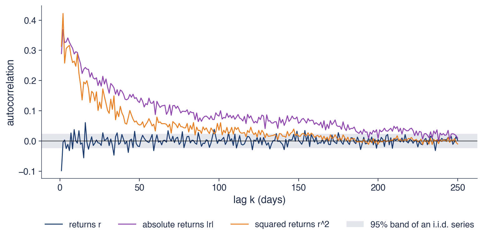
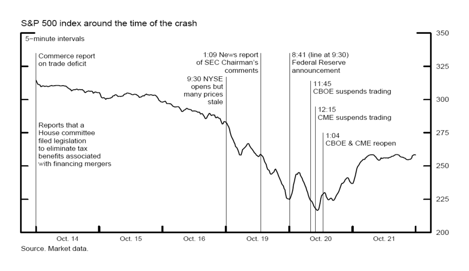


 SFM_ch11_self_similarity