Bucharest University of Economic Studies IDA Institute Digital Assets Blockchain Research Center AI4EFin Artificial Intelligence for Energy Finance Romanian Academy, Institute for Economic Forecasting MSCA Digital Finance
Every later chapter of the course rests on a small set of probability tools. Heavy tails, volatility models, Value at Risk (VaR) and market efficiency are all statements about random variables, their moments, their dependence and the stochastic processes that generate them. This chapter builds these tools from Kolmogorov's axioms up to geometric Brownian motion (GBM), the benchmark model of asset prices, and it tests each of them on real daily data from 2000 to 2026: the S&P 500, the DAX, the BET of the Bucharest Stock Exchange and, from 2014, Bitcoin.
The data repeatedly show where the textbook model fails. On the S&P 500, the empirical VaR 1%, the loss exceeded on 1% of the days, is 3.45%, while a Normal distribution with the same mean and standard deviation gives 2.80%. Daily returns are almost uncorrelated, yet the correlation between today's and yesterday's squared return is 0.31. The standard deviation of today's return rises from 0.91% after the calmest days to 1.71% after the most turbulent ones. These are the features that GBM, with its i.i.d. Normal log returns, cannot produce.
The chapter also introduces simulation. Uniform pseudo-random numbers, the inverse transform and the Monte Carlo method turn any model into an estimate of a probability or an expected value, with a standard error that shrinks like \(1/\sqrt{N}\) in the number of simulations \(N\). The same tools are used in later chapters to price options, to compute portfolio VaR and to test whether a model reproduces the risk of real markets.
Real price paths inside the GBM fan: for the S&P 500 (left), the BET (centre) and Bitcoin (right), the shaded bands contain 90% (light) and 50% (dark) of 4,000 GBM paths calibrated to each series, the dashed line is the GBM median and the dark line is the real price; the price axis is logarithmic.
Learning outcomes
Compute expectations, variances, covariances and correlations, and the volatility of a portfolio.
Explain why uncorrelated returns can still be dependent, and measure this dependence.
Use conditional expectation and conditional variance, the building blocks of GARCH models.
Generate random numbers with the inverse transform and estimate a probability by Monte Carlo, with its standard error.
Define and simulate the binomial model, a random walk, a martingale, white noise, AR(1), the Wiener process and GBM.
Origins of Probability Theory: Games of Chance and Axioms
Probability began as a theory of fair games and became, three centuries later, a branch of measure theory. The section follows this path in four steps. The problem of points, solved by Pascal and Fermat in 1654, introduces the idea that a fair value is an expected value. Kolmogorov's axioms of 1933 give the modern framework, the probability space. Conditional probability and Bayes' rule describe how information changes probabilities, and independence is the case in which it does not.
The section ends with a first test on data: whether a down day on the S&P 500 or on the BET makes another down day more likely. The answer differs between the two markets and anticipates a theme of the whole chapter, the dependence between consecutive returns.
Two players bet on a fair game that ends when one of them has won a fixed number of rounds. If the game is interrupted before the end, how should the stake be divided? The obvious answer, in proportion to the rounds already won, ignores what could still happen. In their correspondence of 1654, Blaise Pascal and Pierre de Fermat proposed instead to divide the stake according to each player's probability of winning the game, had it continued.
In the example on the slide, player A needs one more win and player B needs two. At most two further rounds are needed. B wins the game only by winning both rounds, which in a fair game happens with probability \(1/2 \times 1/2 = 1/4\); in every other case A wins. A should therefore receive 75% of the stake and B 25%. This share is A's expected gain: the stake multiplied by the probability of winning it.
The principle extends far beyond games. The fair price of a contract whose payoff depends on an uncertain future event is an expected payoff, computed under an appropriate probability. This is the logic of derivative pricing: the binomial model of the Binomial Model section prices an option exactly in this way, as an expectation over the up and down paths of the underlying price.
In brief
Two players stop a fair game before the end: how should the stake be split?
Blaise Pascal and Pierre de Fermat solved it in letters (1654): split by the probability of winning, not by the score
Example: A needs 1 more win, B needs 2; at most two more rounds
B wins only if B wins both rounds: probability \(1/4\)
A should get 75% of the stake: its expected gain
The same idea prices a derivative today: a fair price is an expected payoff
For almost three centuries probability had no common foundation. In the Grundbegriffe der Wahrscheinlichkeitsrechnung(Kolmogoroff, 1933), Andrey Kolmogorov placed it on the axioms of measure theory. A probability space is a triple \((\Omega, \mathcal{F}, P)\). The set \(\Omega\) contains all possible outcomes, for example all possible paths of tomorrow's market. The collection \(\mathcal{F}\) is a \(\sigma\)-algebra: the events to which a probability can be assigned, closed under complements and countable unions. The function \(P\) assigns to each event a number in \([0, 1]\).
Three axioms define \(P\). Probabilities are non-negative, \(P(A) \ge 0\); the certain event has probability one, \(P(\Omega) = 1\); and for disjoint events \(A_1, A_2, \dots\), which cannot occur together, the probability that one of them occurs is the sum of their probabilities, \(P(\cup_i A_i) = \sum_i P(A_i)\). The third axiom, countable additivity, is what allows limits: it makes the probability of an event defined by an infinite sequence, such as the convergence of a sample mean, a meaningful quantity.
All the concepts of the chapter follow from these three rules. A random variable is a measurable function on \(\Omega\), its expectation is an integral with respect to \(P\), independence is a factorisation of \(P\), and a stochastic process is a family of random variables on the same probability space.
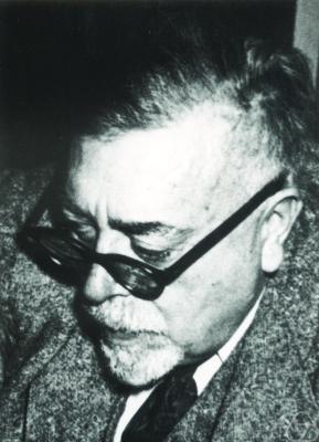
Andrey Nikolaevich Kolmogorov (1903–1987) worked at Moscow State University. His main contribution to probability was to make it a branch of measure theory: events are sets, probability is a measure, and expectations are integrals. This step gave the theory the rigour of analysis and settled the question of what a probability is, mathematically.
His other contributions run through this course. The modern definition of conditional expectation, used in the section on conditioning, is his. He also contributed to the theory of Markov processes and worked on turbulence and on the complexity of sequences. The Kolmogorov–Smirnov test of Chapter 6, which compares an empirical distribution function with a theoretical one, carries his name.
In brief
Andrey Nikolaevich Kolmogorov (1903–1987), Moscow State University
Made probability a branch of measure theory: events are sets, probability is a measure
Also: conditional expectation in its modern form, Markov processes, turbulence, complexity
The Kolmogorov–Smirnov test (Chapter 6) carries his name
The conditional probability of \(A\) given \(B\), for \(P(B) > 0\), is
\[P(A \mid B) = \frac{P(A \cap B)}{P(B)},\]
(4.1)
where \(A \cap B\) is the event that both occur. In words, among the cases in which \(B\) occurs, \(P(A \mid B)\) is the share in which \(A\) also occurs. Conditioning restricts the probability space to \(B\) and rescales \(P\) so that the restricted space has total probability one.
Bayes' rule reverses the direction of conditioning:
\[P(B \mid A) = \frac{P(A \mid B)\,P(B)}{P(A)}.\]
(4.2)
Here \(P(B)\) is the probability of \(B\) before \(A\) is observed, the prior, and \(P(B \mid A)\) is the updated probability once \(A\) is known, the posterior. The typical financial use is a warning signal: from the probability that the signal appears given a crisis, Bayes' rule gives the probability of a crisis given that the signal has appeared, which also depends on how frequent crises and false signals are.
Two events are independent if \(P(A \cap B) = P(A)P(B)\), which is equivalent to \(P(A \mid B) = P(A)\) when \(P(B) > 0\): learning that \(B\) occurred does not change the probability of \(A\). Independence is a property of the probability measure, not of the events themselves, and it is the assumption behind most of the simple models of the chapter, from the binomial tree to GBM.
In brief
Conditional probability: \(P(A \mid B) = P(A \cap B)/P(B)\), for \(P(B) > 0\)
\(A, B\): two events; \(A \cap B\): both occur
in words: among the cases in which \(B\) occurs, the share in which \(A\) also occurs
Bayes' rule: \(P(B \mid A) = P(A \mid B)P(B)/P(A)\)
\(P(B)\): the probability of \(B\) before we learn \(A\); \(P(B \mid A)\): the updated probability once \(A\) is observed
it reverses the direction of conditioning: from “signal given crisis” to “crisis given signal”
Independent events: \(P(A \cap B) = P(A)P(B)\), i.e. \(P(A \mid B) = P(A)\)
learning that \(B\) occurred does not change the probability of \(A\)
The definitions can be tested on daily index returns. For the S&P 500 between 2000 and 2026, the share of down days is 46.3%. After a down day, the frequency of another down day is 43.4%, slightly lower. Two down days in a row occur on 20.1% of the pairs of consecutive days; under independence the probability would be \(0.463^2 = 21.4\%\). The difference is small, and as a first approximation the sign of the S&P 500 return is close to independent from one day to the next.
The BET behaves differently. After a down day the probability of another down day is 50.0%, against 42.6% after an up day: the sign of the return persists. The usual explanation is thin trading. On a market with fewer trades and less liquid stocks, prices adjust to news over several days instead of at once, so a fall today tends to be followed by a further adjustment tomorrow. The same effect appears below as a positive first-order autocorrelation of BET returns.
A probability model is a probability space \((\Omega, \mathcal{F}, P)\), and the three axioms of Kolmogorov fix the rules for \(P\). The idea of Pascal and Fermat, that a fair value is an expected value, will return in the binomial model and in option pricing.
Conditional probability measures how information changes the odds, and Bayes' rule reverses the direction of conditioning. On daily data the S&P 500 is close to sign independence, while the BET shows persistence, a first sign that consecutive returns need not be independent.
In brief
Probability space \((\Omega, \mathcal{F}, P)\) and three axioms
Fair value = expected value: the idea of Pascal and Fermat
Conditional probability measures how information changes the odds
Section summary
The section has set the framework for the rest of the chapter: outcomes, events and a probability measure that satisfies three axioms. Conditional probability and independence are the first tools for dependence between events. The next section attaches numbers to outcomes, through random variables, and describes their distributions.
Random Variables and Distributions
A random variable turns the outcomes of a probability space into numbers: tomorrow's log return, the number of up days in a week, the loss of a portfolio. Its distribution is described by a probability mass function (PMF) in the discrete case, by a probability density function (PDF) in the continuous case, and by the cumulative distribution function (CDF) in both. The inverse of the CDF, the quantile function, gives the Value at Risk.
The section then turns to data. It compares the weekly count of up days of the S&P 500 with a binomial distribution, and the empirical CDF of daily returns with the Normal CDF, with special attention to the left tail, where risk is measured.
A random variable is a function \(X: \Omega \to \mathbb{R}\) that assigns a number to each outcome (measurable with respect to \(\mathcal{F}\), so that events such as \(\{X \le x\}\) have a probability). Tomorrow's log return, the number of up days in a week and the loss of a portfolio over a month are all random variables defined on the same probability space as the market outcomes.
A random variable is discrete if it takes finitely or countably many values \(x_i\). Its distribution is given by the PMF (probability mass function), \(p(x_i) = P(X = x_i)\), with \(\sum_i p(x_i) = 1\). The number of up days in a week is discrete, with values 0 to 5.
A random variable is continuous if probabilities of intervals are areas under a density: \(P(a < X \le b) = \int_a^b f(x)\,dx\). The function \(f\) is the PDF (probability density function), with \(f \ge 0\) and total area \(\int f = 1\). A single point has zero area, so \(P(X = x) = 0\) for every \(x\): for a continuous return, only intervals of values have positive probability. The density is not itself a probability and can exceed one. The textbook treatment is in Franke, Härdle & Hafner (2019), Sec. 3.1.
In brief
A random variable\(X: \Omega \to \mathbb{R}\) assigns a number to each outcome
tomorrow's log return, the number of up days in a week, the loss of a portfolio
Discrete: finitely or countably many values \(x_i\)
PMF (probability mass function): \(p(x_i) = P(X = x_i)\), with \(\sum_i p(x_i) = 1\)
\(p(x_i)\): the probability of the value \(x_i\); the probabilities of all values add up to 1
Continuous: \(P(a < X \le b) = \int_a^b f(x)\,dx\)
the probability of an interval \((a, b]\) is the area under \(f\) between \(a\) and \(b\)
\(f\) is the PDF (probability density function): \(f \ge 0\) and the total area \(\int f = 1\)
a single point has no area: \(P(X = x) = 0\) for every \(x\)
The CDF (cumulative distribution function) of \(X\) is \(F(x) = P(X \le x)\), the probability that \(X\) does not exceed the threshold \(x\). Every CDF is non-decreasing and right-continuous, and rises from \(F(-\infty) = 0\) to \(F(\infty) = 1\). The CDF exists for every random variable, discrete or continuous, which makes it the common language of the chapter. For a continuous \(X\), the density is its derivative, \(f = F'\).
The quantile of order \(\alpha \in (0, 1)\) inverts the CDF:
the smallest \(x\) for which \(P(X \le x) \ge \alpha\). The infimum makes the definition work also where \(F\) has jumps or flat parts, where an ordinary inverse does not exist. The function \(\alpha \mapsto F^{-1}(\alpha)\) is the quantile function.
Two quantiles appear throughout the course. The median is \(q_{0.5}\), the value that splits the distribution in two halves. The 1% quantile of daily returns is the return exceeded on 99% of the days: a negative number, which measures how bad a bad day is.
In brief
CDF (cumulative distribution function): \(F(x) = P(X \le x)\)
the probability that \(X\) does not exceed the threshold \(x\)
non-decreasing, right-continuous, from \(F(-\infty) = 0\) to \(F(\infty) = 1\)
for a continuous \(X\) the density is its derivative: \(f = F'\)
Quantile of order \(\alpha\): \(q_\alpha = F^{-1}(\alpha) = \inf\{x : F(x) \ge \alpha\}\)
\(\alpha \in (0, 1)\): a probability; \(q_\alpha\) is the smallest \(x\) with \(P(X \le x) \ge \alpha\)
\(F^{-1}\): the quantile function, the inverse of the CDF; \(\inf\): the smallest value of the set
median \(= q_{0.5}\); the 1% quantile is the return exceeded on 99% of the days
VaR (Value at Risk) at level 1% is minus the 1% quantile of the returns:
\[\text{VaR}_{1\%} = -q_{0.01}.\]
(4.4)
The quantile \(q_{0.01}\) is negative for daily returns, and the minus sign turns it into a positive loss: VaR 1% is the loss exceeded with probability 1%. The course writes the level as the tail probability, VaR 1% or VaR 5%, so that \(\text{VaR}_\alpha = -q_\alpha\). Estimation and backtesting of VaR are the subject of Chapter 10.
In practice \(F\) is unknown and is estimated from data. For observed returns \(r_1, \dots, r_n\), the empirical CDF is
\[\hat F(x) = \frac1n\,\#\{t : r_t \le x\},\]
the share of days with a return at most \(x\);\(\#\{\cdot\}\) counts the days in the set, and the hat marks an estimate. \(\hat F\) is a step function that jumps by \(1/n\) at each observation. Its quantiles are the sorted returns, and the empirical VaR 1% is minus the return below which 1% of the days lie.
In brief
VaR (Value at Risk) 1%: \(\text{VaR}_{1\%} = -q_{0.01}\)
\(q_{0.01}\): the 1% quantile of the returns, a negative number
the minus sign turns it into a loss: the loss exceeded with probability 1%
Conditional probabilities of the event D, daily log returns
Question for the room For the S&P 500, P(down today | down yesterday) = 43.4% is even below P(down) = 46.3%. The ▶ button raises the threshold x: the event D becomes a loss of more than x%. At x = 2%, what is P(D | D yesterday) against P(D) = 4.27%?
Answer
11.85%, 2.8 times P(D). Two losses of more than 2% in a row have a frequency of 0.51%, against 0.18% under independence. The sign of the return barely persists for the S&P 500, but large losses come in clusters: volatility clustering. For BET the sign persists too, at x = 0: 50.0% after a down day against 42.6% after a day that is not down, an effect of thin trading.
Question for the room For the S&P 500, the variance of K (1.16) is slightly below the binomial variance 5p(1 − p) = 1.24. The ▶ button moves to the DAX and BET. What happens for BET, whose daily return has a first-order autocorrelation of 0.109?
Answer
The variance of K exceeds the binomial value: 1.47 against 1.24, ratio 1.18. The binomial distribution assumes independent days; with the positive autocorrelation of BET returns, up days come one after another more often, so weeks with many or with few up days are more frequent. The mean stays close to 5p: 2.67 against 2.70. For the S&P 500, with autocorrelation −0.099, the ratio is 0.93; for the DAX also 0.93.
The left panel shows a discrete random variable, \(K\), the number of up days in a full five-day week of the S&P 500, computed over 1,144 weeks. The dark bars are the frequencies in the data and the light bars the binomial distribution \(B(5, p)\), which assumes five independent days, each up with probability \(p = 0.537\). The two sets of bars are close: the mean of \(K\) is 2.67 in the data against 2.69 for the binomial, and the variance is 1.16 against 1.24.
The right panel shows a continuous random variable, the daily log return. The histogram estimates the PDF and is compared with the Normal density with the same mean and standard deviation. The Normal curve misses the shape of the data in two places: the empirical density has a much higher, narrower peak around zero, and its tails extend far beyond the region where the Normal density is practically zero.
The contrast between the two panels anticipates a theme of the course. Counting up and down days discards the size of the moves, and for this count the independent binomial model works well. The size of the moves is where the Normal model fails; the heavy tails and the high peak are the stylised facts of Chapter 2.
In brief
Left: \(K\) = number of up days in a full week of the S&P 500 (1 144 weeks)
compared with \(B(5, p)\), the binomial distribution: 5 days, each up with probability \(p = 0.537\)
mean 2.67 vs 2.69; variance 1.16 vs 1.24
Right: daily log returns, a continuous random variable; the histogram estimates the PDF
The binomial fits \(K\) well; the Normal density misses the peak and the tails of the returns (Chapter 2)
Question for the room Bitcoin trades every day, so the chapter annualises with A = 365. The daily standard deviation is 3.485%. What is the annual volatility?
Answer
66.6% = 3.485 × √365. With A = 252, as for stocks, it would be 55.3%. The annual mean is 43.1% with A = 365 (29.8% with A = 252). The volatility grows with √A, the mean with A, and both assume i.i.d. returns. The excess kurtosis of 11.96 shows that the daily distribution is not Normal, even though the square-root-of-time rule uses only the variance.
Days with |r − mean| > kσ: data, the Normal distribution and Chebyshev's bound
Worked example: Chebyshev's bound against the data
Question for the room For k = 2, Chebyshev's inequality allows up to 25% of the days. What share of the S&P 500 days lies more than 2 standard deviations from the mean?
Answer
4.90% (329 days), close to 4.55% under the Normal distribution. At 2 standard deviations the data look like the Normal distribution; the difference is in the tail: at k = 4 there are 46 days (0.69%), 108 times the 0.0063% of the Normal distribution, and at k = 6 there are 12 days, against 1.3 × 10⁻⁵ expected days. Chebyshev's bound, 1/k², holds for any distribution with finite variance, which is why it lies far above the data.
Question for the room At the 1% level, the empirical VaR of the S&P 500 (3.45%) is 1.24 times the VaR of the Normal distribution with the same mean and standard deviation (2.80%). The ▶ button lowers the level α from 5% to 0.1%. What does the ratio become at α = 0.1%?
Answer
About 1.94: VaR 0.1% is 7.22% in the data and 3.72% under the Normal distribution. At α = 5% the ratio is 0.94 (1.85% against 1.97%). If the difference were only one of scale, the ratio would be the same at every level; it grows towards the tail, so the problem is the shape of the distribution: a higher peak and heavier tails. P(r < −5%) is 0.34% in the data and 1.7 × 10⁻³% under the Normal distribution, 199 times less.
The left panel compares the empirical CDF of 6,714 daily log returns of the S&P 500 with the Normal CDF with the same mean and standard deviation. On the linear scale the curves look similar. The median daily return is 0.063%, and \(\hat F(0) = 46.3\%\): on 46.3% of the days the return was not positive. The right panel shows the left tail on a logarithmic vertical axis, where the difference becomes visible. The horizontal dotted line marks the 1% level, and the two vertical lines the empirical and the Normal 1% quantile.
The empirical VaR 1% is 3.45%, while the Normal VaR 1% is 2.80%: the Normal model understates the loss exceeded on 1% of the days. Deeper in the tail the gap widens. A daily fall of more than 3% occurred on 1.55% of the days, against 0.63% under the Normal distribution. A fall of more than 5% occurred on 0.34% of the days, 199 times the Normal probability of \(1.7 \times 10^{-3}\%\).
On the log scale the empirical tail decays slowly, while the Normal tail bends down sharply, like \(e^{-x^2/2}\). For any distribution with tails heavier than Normal, the ratio of the two tail probabilities therefore grows without limit as the threshold moves further into the tail. Any risk measure computed from a Normal model inherits this error, which is why later chapters model the tails directly.
In brief
\(n = 6\,714\) days; median \(0.063\%\); \(\hat F(0) = 46.3\%\) of the days are not up days
VaR 1%: empirical 3.45%, Normal 2.80%; \(P(r < -3\%)\): 1.55% vs 0.63%
\(P(r < -5\%)\): 0.34% in the data, 199 times the value under the Normal distribution (\(1.7 \times 10^{-3}\%\))
A discrete random variable is described by its PMF and a continuous one by its PDF; the CDF describes both. Quantiles invert the CDF, and VaR 1% is minus the 1% quantile of the returns, \(\text{VaR}_{1\%} = -q_{0.01}\).
On the S&P 500, the number of up days per week is well described by a binomial distribution, but the size of daily returns is not Normal. The empirical tail is much heavier: a fall of more than 5% is about two hundred times more frequent than the Normal distribution predicts.
In brief
PMF for discrete, PDF for continuous variables; the CDF works for both
Quantiles invert the CDF; VaR 1% is minus the 1% quantile
The tails of the empirical CDF are much heavier than the Normal ones
Section summary
Random variables, their CDFs and their quantiles are the objects on which risk measures are defined. The first comparison with data has shown that the Normal distribution describes the centre of daily returns acceptably but understates the left tail. The next section summarises distributions by their moments: the mean, the variance and the higher moments that measure asymmetry and tail weight.
Expectation and Variance
A distribution is often summarised by a few numbers. The expectation locates its centre, the variance measures its spread, and the third and fourth moments measure asymmetry and tail weight. This section defines these moments, states the rules by which they combine, and applies them to two questions on S&P 500 data: how daily figures scale to a year, and how rare a day four standard deviations from the mean really is.
the sum of the values weighted by their probabilities in the discrete case, and the integral against the density in the continuous case. Geometrically it is the centre of mass of the distribution. It exists only if \(E|X| < \infty\). The Cauchy distribution, a stable law of Chapter 3, has tails so heavy that this integral diverges, and it has no mean. The expectation of a function of \(X\) is computed directly as \(E[g(X)] = \int g(x) f(x)\,dx\), without first deriving the distribution of \(g(X)\).
The most useful property of expectation is linearity:
\[E[aX + bY + c] = a\,E[X] + b\,E[Y] + c,\]
(4.5)
for constants \(a, b, c\) and any random variables \(X\) and \(Y\), dependent or not. It follows that the expected return of a portfolio is the weighted mean of the expected returns of its assets, with the portfolio weights as weights, whatever the dependence between the assets.
Linearity does not extend to nonlinear functions: in general \(E[g(X)] \ne g(E[X])\).Jensen's inequality gives the direction for a convex \(g\):\(E[g(X)] \ge g(E[X])\), with strict inequality unless \(X\) is constant. For example \(E[e^X] > e^{E[X]}\). With \(X\) a log return, \(e^X\) is the gross simple return, so the mean simple return exceeds the exponential of the mean log return. This gap is the volatility drag of Chapter 1, and it reappears below as the difference between the mean and the median of GBM.
In brief
Expectation (mean): \(E[X] = \sum_i x_i p(x_i)\) or \(E[X] = \int x f(x)\,dx\)
\(x_i\), \(p(x_i)\): the values and their probabilities; \(f\): the density
the centre of mass of the distribution; it exists only if \(E|X| < \infty\) (not for Cauchy, Chapter 3)
Of a function: \(E[g(X)] = \int g(x) f(x)\,dx\), without finding the distribution of \(g(X)\)
Linearity: \(E[aX + bY + c] = aE[X] + bE[Y] + c\), always (no independence needed)
\(a, b, c\): constants; \(X, Y\): any two random variables
the expected return of a portfolio is the weighted mean of the expected returns
In general \(E[g(X)] \ne g(E[X])\)
Jensen: for a convex \(g\), \(E[g(X)] \ge g(E[X])\); for example \(E[e^X] > e^{E[X]}\)
The second form follows from expanding the square and using linearity. The standard deviation\(\sigma = \sqrt{\text{Var}(X)}\) is measured in the units of \(X\); for returns it is called volatility. Adding a constant does not change risk and multiplying by a constant multiplies the variance by its square: \(\text{Var}(aX + b) = a^2\,\text{Var}(X)\). A position twice as large has twice the volatility and four times the variance.
The moments of \(X\) are \(E[X^k]\),\(k = 1, 2, \dots\); the central moments use \(X - \mu\). Two standardised central moments describe the shape of a distribution. The skewness\(E[(X - \mu)^3]/\sigma^3\) measures asymmetry and is zero for any symmetric distribution, the Normal distribution included. The kurtosis\(E[(X - \mu)^4]/\sigma^4\) measures the weight of the tails relative to the centre and equals 3 for the Normal distribution.
The excess kurtosis, kurtosis minus 3, is therefore zero for the Normal distribution and positive for distributions with heavy tails. Daily returns of stock indices have excess kurtosis around 10, as the section on GBM shows, and Chapter 2 studies this fact in detail.
The example converts daily moments of S&P 500 log returns into annual ones. Over 2000–2026, the daily mean log return is 0.0247% and the daily standard deviation is \(\sigma = 1.213\%\); a year has \(A = 252\) trading days. Assume that daily returns are i.i.d., independent and identically distributed. Log returns add over time, so the annual log return is the sum of the \(A\) daily ones, \(\sum_{t=1}^{A} r_t\).
By linearity of expectation, the annual mean is \(A\) times the daily mean: \(252 \times 0.0247\% = 6.2\%\) a year. For the variance, the variance of a sum equals the sum of the variances plus twice all covariances, as (4.7) in the next section shows; under independence the covariances are zero, so \(\text{Var}(\sum r_t) = A\sigma^2\). The annual volatility is \(\sigma\sqrt{A} = 1.213\% \times \sqrt{252} = 19.3\%\).
This is the square-root-of-time rule: over \(h\) periods the mean grows like \(h\) and the volatility like \(\sqrt{h}\). It is used everywhere to annualise volatility and to scale a one-day VaR to longer horizons. It depends on the absence of autocorrelation; with persistent returns, positive autocorrelations make the variance of the sum larger than \(h\sigma^2\), and negative ones make it smaller.
In brief
S&P 500, daily log returns \(r_t\)
daily mean \(0.0247\%\), daily standard deviation \(\sigma = 1.213\%\)
\(A = 252\): the number of trading days per year
Assume i.i.d. daily returns (independent and identically distributed)
the annual log return is the sum of the \(A\) daily ones: \(\sum_{t=1}^{A} r_t\)
Mean: \(E[\sum r_t] = A \times 0.0247 = 6.2\%\) a year
linearity of expectation
Variance: \(\text{Var}(\sum r_t) = A\,\sigma^2\), because the covariances are zero
Chebyshev's inequality bounds the probability of a large deviation using only the mean and the variance. For any \(X\) with finite variance and any \(k > 1\),
\[P(|X - \mu| \ge k\sigma) \le \frac{1}{k^2},\]
(4.6)
where \(k\) is the distance from the mean in standard deviations. Because it uses only two moments, the bound holds for every distribution; the price of this generality is that it is usually far from tight.
For \(k = 4\) and the S&P 500 over 2000–2026, the three answers are very different. Chebyshev allows at most \(1/16 = 6.25\%\) of the days to lie four or more standard deviations from the mean. The Normal distribution gives 0.0063%. The data contain 46 such days, 0.69% of the sample.
The data lie between the two extremes. The Normal distribution is far too optimistic: 4-sigma days are far more frequent in the data than it predicts. Chebyshev's worst case, valid for every distribution with finite variance, is too pessimistic. A useful model of returns must sit in between, with tails heavier than Normal but lighter than the worst case, which is the task of the heavy-tailed distributions of Chapter 5.
In brief
Chebyshev's inequality: for any \(X\) with finite variance, \(P(|X - \mu| \ge k\sigma) \le 1/k^2\)
\(\mu\), \(\sigma\): the mean and the standard deviation; \(k > 1\): the distance from the mean, in standard deviations
it uses only the mean and the variance, so it holds for every distribution
\(k = 4\), S&P 500, 2000–2026
Chebyshev bound: at most 6.25% of the days
Normal distribution: 0.0063%
data: 46 days, 0.69%
The data lie between the two
the Normal distribution is far too optimistic; the worst case of Chebyshev is too pessimistic
Expectation is linear for any random variables, while variance scales with the square of a constant. Jensen's inequality explains why the mean of a convex function exceeds the function of the mean, the origin of the volatility drag.
For i.i.d. returns the mean grows in proportion to the horizon \(h\) and the volatility in proportion to \(\sqrt{h}\). Chebyshev's inequality bounds tail probabilities for any distribution; on the S&P 500 the frequency of 4-sigma days lies between this bound and the much smaller Normal value.
In brief
Expectation is linear; variance scales with the square
For i.i.d. returns the mean grows with \(h\) and the volatility with \(\sqrt{h}\)
Chebyshev bounds tail probabilities for any distribution
Section summary
The first two moments summarise location and spread, and the standardised third and fourth moments summarise asymmetry and tail weight. The examples of the section treated one series at a time and assumed independent days. The next section studies several random variables together, through their joint distribution, and measures the dependence between them.
Joint Distributions and Dependence
Portfolios, hedges and contagion all involve several random variables at once. Their joint distribution contains more information than the separate (marginal) distributions: it also says how the variables move together. This section defines the joint and marginal distributions, the covariance and the correlation, and the variance of a sum, which gives the risk of a portfolio. It then separates two notions that are often confused, uncorrelatedness and independence, and shows on data that daily returns are nearly uncorrelated but far from independent.
For two random variables \(X\) and \(Y\), the joint CDF is \(F(x, y) = P(X \le x, Y \le y)\), the probability that both variables lie below their thresholds at the same time. For two daily returns it is the probability that both markets fall below given levels on the same day, the quantity that matters for a joint crash.
The marginal CDF of \(X\) is obtained by letting the other threshold go to infinity: \(F_X(x) = F(x, \infty)\). It is the distribution of \(X\) alone, whatever the value of \(Y\). The marginals can be recovered from the joint distribution, but not the other way round: many joint distributions share the same marginals and differ only in their dependence.
If \((X, Y)\) has a joint PDF\(f(x, y)\), the probability of any region \(B\) of the plane is the volume under \(f\) above \(B\):
\[P((X, Y) \in B) = \iint_B f(x, y)\,dx\,dy.\]
The marginal density of \(X\) follows by integrating \(Y\) out, \(f_X(x) = \int f(x, y)\,dy\).
In brief
Joint CDF: \(F(x, y) = P(X \le x, Y \le y)\)
the probability that both variables are below their thresholds at the same time
for two returns: both markets fall below given levels on the same day
Marginal CDF: \(F_X(x) = F(x, \infty)\)
the distribution of \(X\) alone, whatever the value of \(Y\)
where \(\mu_X\) and \(\mu_Y\) are the means. It is positive when \(X\) and \(Y\) tend to be above their means at the same time and negative when one tends to be above while the other is below. Its unit is the product of the units of \(X\) and \(Y\), so its size is hard to interpret directly.
The correlation removes the units by dividing by the two standard deviations, \(\rho = \text{Cov}(X, Y)/(\sigma_X\sigma_Y)\), and always lies in \([-1, 1]\). It measures linear dependence only: \(|\rho| = 1\) if and only if \(Y = a + bX\) for constants \(a\) and \(b \ne 0\). A correlation close to zero rules out a linear relation, not every relation, which is the subject of the frame on independence.
In a portfolio, \(a\) and \(b\) are the weights. The covariance term can raise or lower the risk: with positive weights, a negative or small covariance reduces the portfolio variance below what the separate variances would suggest. For \(N\) assets the formula becomes \(\sigma_p^2 = w^\top \Sigma w\), where \(w\) is the vector of weights, \(w^\top\) its transpose and \(\Sigma\) the \(N \times N\) covariance matrix, which contains the variances on the diagonal and the covariances off the diagonal.
Question for the room The ▶ button moves the weight a of the S&P 500 in the S&P 500/DAX portfolio from 0 to 1. At which weight is the volatility of the portfolio lowest?
Answer
At a* = (σ2² − Cov)/(σ1² + σ2² − 2Cov) = 0.69, with σp = 1.163%, against 1.186% at a = 0.5. The S&P 500 gets the larger weight because its volatility is lower (1.221% against 1.429%), but not 1: with ρ = 0.60, some DAX still reduces the risk. For S&P 500/BET, with ρ = 0.21: a* = 0.60 and σp = 1.025%.
Question for the room The daily correlation of the S&P 500 and BET over the whole period is 0.21. What is it on the days of 2020?
Answer
0.63, on 242 common days, three times the value over the whole period. In 2008 the correlation is 0.28, in 2017 0.20. For the S&P 500 and the DAX: 0.69 in 2020, 0.62 in 2008 and 0.57 in 2017, against 0.60 over the whole period. Correlation rises in crisis years, exactly when diversification would be needed.
The two scatter plots show pairs of daily log returns on common trading days. Markets have different holidays, so the prices are first matched on the dates when both markets traded and the returns are then computed from the matched prices; for the S&P 500 and the DAX this gives 6,605 days. Each point is one day, with the S&P 500 return on the horizontal axis and the DAX (left) or BET (right) return on the vertical axis.
The S&P 500 and the DAX have correlation 0.60: the cloud is clearly tilted along the diagonal. The S&P 500 and the BET have correlation 0.21, and the cloud is much rounder: the two markets share fewer common shocks on the same day.
In the centre, both clouds are roughly elliptical, the shape a bivariate Normal distribution would produce. The extreme points tell a different story: the largest falls and rises tend to occur on the same days in both markets, along the diagonal. Crises hit all markets together, so the dependence in the tails is stronger than the correlation, computed mostly from ordinary days, suggests.
In brief
Common trading days only: prices are joined first, then differenced (\(n = 6\,605\) days for S&P 500 and DAX)
S&P 500 and DAX: \(\rho = 0.60\); S&P 500 and BET: \(\rho = 0.21\)
The cloud is elliptic in the centre, but extreme days are joint: crises hit all markets together
Apply (4.7) to a portfolio with half of its value in each index. The daily standard deviations are \(\sigma_1 = 1.22\%\) for the S&P 500 and \(\sigma_2 = 1.43\%\) for the DAX, the covariance is 1.045 (in squared percent) and the correlation 0.60. With weights \(a = b = 0.5\),\(a^2 = b^2 = 0.25\) and \(2ab = 0.5\).
The variance terms contribute \(0.25\sigma_1^2 + 0.25\sigma_2^2 = 0.883\) and the covariance term \(0.5 \times 1.045 = 0.522\), so \(\sigma_p^2 = 1.405\) and the portfolio volatility is \(\sigma_p = 1.19\%\) a day. The average volatility of the two indices is 1.32%. The difference is the diversification effect: because \(\rho < 1\), the portfolio is less risky than the average of its parts. The same calculation for the S&P 500 and the BET, which have a lower correlation, gives a portfolio volatility of 1.04% against an average of 1.33%: the lower the correlation, the larger the reduction in risk.
Diversification works only through \(\rho < 1\); with \(\rho = 1\) the portfolio volatility equals the weighted average of the volatilities. The difficulty is that correlations are not constant. In a crash correlations rise, as the scatter plots of the previous frame suggest, so the risk reduction shrinks exactly when it is needed most.
Two random variables \(X\) and \(Y\) are independent if their joint CDF factorises, \(F(x, y) = F_X(x)F_Y(y)\) for all \(x\) and \(y\). Independence is much stronger than zero correlation: it implies \(E[g(X)h(Y)] = E[g(X)]E[h(Y)]\) for all functions \(g\) and \(h\) for which the expectations exist, for example squares or absolute values. Taking \(g\) and \(h\) equal to the identity gives \(E[XY] = E[X]E[Y]\), that is, zero covariance. Independent variables are therefore uncorrelated.
The converse is false. Take \(X \sim N(0, 1)\) and \(Y = X^2\). Then \(\text{Cov}(X, X^2) = E[X^3] - E[X]E[X^2] = 0\), because the odd moments of a symmetric distribution vanish: \(X\) and \(Y\) are uncorrelated. But \(Y\) is a function of \(X\), so once \(X\) is known \(Y\) is known exactly: the dependence is complete. Correlation misses it because the relation is not linear; it is symmetric, and the positive and negative values of \(X\) cancel.
There is one important exception. If \(X\) and \(Y\) are jointly Normal, zero correlation implies independence, because the joint Normal density factorises when the covariance is zero. This is why models built on the Normal distribution can treat correlation as a complete description of dependence, and why this description fails for returns, which are not jointly Normal.
In brief
\(X\) and \(Y\) are independent if \(F(x, y) = F_X(x)F_Y(y)\) for all \(x, y\)
the joint CDF is the product of the marginal CDFs
then \(E[g(X)h(Y)] = E[g(X)]E[h(Y)]\) for all functions \(g, h\) (for example squares or absolute values)
Independent \(\Rightarrow\) uncorrelated (\(g, h\) = identity); the converse is false
Example: \(X \sim N(0, 1)\), \(Y = X^2\)
\(\text{Cov}(X, X^2) = E[X^3] = 0\): uncorrelated
but \(Y\) is a function of \(X\): completely dependent
Exception: for jointly Normal variables, uncorrelated \(\Leftrightarrow\) independent
Question for the room The ▶ button raises the lag h from 1 to 20. At h = 20, is Corr(rt², rt−20²) of the S&P 500 still outside the band ±1.96/√n = ±0.024?
Answer
Yes: 0.164 at lag 20, against 0.313 at lag 1, while the correlation of the returns at lag 20 is 0.014, inside the band. At lag 1, the correlation of the squares is 0.31 (S&P 500), 0.15 (DAX), 0.33 (BET) and 0.14 (Bitcoin). At lag 20 it stays above the band for the DAX (0.116) and BET (0.090); for Bitcoin (0.026) it falls inside the band ±0.030. Volatility clustering lasts for weeks. The band is an asymptotic reference value for an i.i.d. series, not an exact test at every lag.
The left panel shows simulated pairs \((X, X^2)\) with \(X\) standard Normal. The points lie exactly on a parabola, yet the sample correlation is \(-0.038\), close to zero. The figure makes the previous frame concrete: perfect dependence, no correlation.
The right panel shows the same phenomenon in real data. For each series, the dark bar is the first-order autocorrelation of daily returns, \(\text{Corr}(r_t, r_{t-1})\), and the light bar the first-order autocorrelation of squared returns, \(\text{Corr}(r_t^2, r_{t-1}^2)\). The dashed lines mark the band \(\pm 1.96/\sqrt{n}\): the values compatible with zero correlation at the 5% level for an i.i.d. series of length \(n\). The return autocorrelations are small: \(-0.099\) for the S&P 500, \(-0.017\) for the DAX and \(-0.022\) for Bitcoin. The negative S&P 500 value comes mostly from crisis days, when large moves were followed by partial reversals.
The squared returns behave very differently. Their autocorrelations, 0.31 for the S&P 500, 0.15 for the DAX, 0.14 for Bitcoin and 0.33 for the BET, are far outside the band: a large move today, of either sign, is followed by a large move tomorrow. This is volatility clustering, and it shows that daily returns are dependent although almost uncorrelated. The BET is the exception for the returns themselves: \(\text{Corr}(r_t, r_{t-1}) = 0.109\), the positive autocorrelation produced by thin trading, which the down-day example of the first section already showed.
In brief
Left: simulated \(Y = X^2\), sample correlation \(-0.038\), yet \(Y\) is determined by \(X\)
The covariance enters the variance of every portfolio through (4.7); correlation below one is the source of diversification, and its rise in crises is its limit. Independence implies zero correlation, but zero correlation does not imply independence, except for jointly Normal variables.
Daily returns are nearly uncorrelated, but their squares are clearly correlated, so returns are not independent. The dependence is in the size of the moves, not in their direction, which motivates the conditional variance of the next section.
In brief
Covariance enters the variance of every portfolio
Independent implies uncorrelated, not the other way round
Returns: nearly uncorrelated, but their squares are correlated, so they are not independent
Section summary
Correlation describes the linear part of the dependence between two variables. It governs portfolio variance, but it misses the dependence of returns through their magnitude, visible in the autocorrelation of squared returns. The next section describes this dependence directly, by conditioning on the past: the conditional mean and the conditional variance.
Conditional Expectation and Conditional Variance
Forecasting means conditioning: replacing the unconditional distribution of tomorrow's return by its distribution given what is known today. This section defines the conditional expectation, the best forecast in the mean-squared sense, and the conditional variance, which measures the remaining uncertainty. The law of total variance splits total risk into a part within groups of similar conditions and a part between them. On S&P 500 and Bitcoin data, conditioning on the size of yesterday's move barely changes the mean of today's return, but changes its standard deviation substantially. This finding leads directly to the ARCH and GARCH models.
If \((X, Y)\) has a joint density, the conditional density of \(Y\) given \(X = x\) is \(f(y \mid x) = f(x, y)/f_X(x)\): the slice of the joint density at \(X = x\), rescaled by the marginal density so that it integrates to one. It is the distribution of \(Y\) once it is known that \(X = x\). The conditional expectation is the mean of this distribution,
\[E[Y \mid X = x] = \int y\,f(y \mid x)\,dy.\]
As a function of the random \(X\),\(E[Y \mid X]\) is itself a random variable.
The conditional expectation is the best forecast of \(Y\) from \(X\): among all functions \(g\), it minimises the mean squared error \(E[(Y - g(X))^2]\). For returns the conditioning information is usually the whole past. Writing \(\mathcal{F}_{t-1}\) for all information available up to yesterday, \(E[r_t \mid \mathcal{F}_{t-1}]\) is the forecast of today's return given that information.
The tower property, or law of iterated expectations, states that
\[E\big[E[Y \mid X]\big] = E[Y].\]
(4.8)
Averaging the conditional forecasts over all values of \(X\) gives back the unconditional mean. A forecast that is sometimes high and sometimes low must be right on average.
Like the conditional mean, it is a random variable, a function of \(X\). For returns, \(\text{Var}(r_t \mid \mathcal{F}_{t-1})\) is the variance of today's return given the past, the quantity that volatility models forecast.
The law of total variance decomposes the unconditional variance:
The first term is the average variance inside the groups defined by \(X\), the within-group variance. The second is the variance of the group means, the between-group variance: how much the conditional means differ from each other. The identity follows from the tower property applied to \(Y^2\) and to \(Y\).
The decomposition answers a practical question: is risk driven by changes in the expected return or by changes in the dispersion around it? If the between part is small, knowing \(X\) barely improves the forecast of \(Y\) itself, but it can still change the forecast of its variance.
Let \(X\) be the market regime and \(Y = r\) the daily return, in percent. The calm regime has probability 0.7, mean 0.05% and standard deviation 0.8%; the turbulent regime has probability 0.3, mean \(-0.10\%\) and standard deviation 2%. The unconditional distribution of \(r\) is a mixture of two Normal-like distributions.
By the tower property (4.8), the unconditional mean is the probability-weighted mean of the regime means: \(E[r] = 0.7 \times 0.05 + 0.3 \times (-0.10) = 0.005\%\). For the variance, (4.9) gives two parts. The within part is \(E[\text{Var}(r \mid X)] = 0.7 \times 0.8^2 + 0.3 \times 2^2 = 1.648\). The between part is \(\text{Var}(E[r \mid X]) = 0.7(0.05 - 0.005)^2 + 0.3(-0.10 - 0.005)^2 = 0.0047\). The total variance is 1.653, and the standard deviation is 1.286%.
Almost all the risk comes from the different variances of the regimes, not from their different means. The example also shows why such mixtures have heavy tails: most days are drawn from the calm distribution, which produces a high, narrow peak, and some from the turbulent one, which produces large moves.
In brief
\(X\) = the market regime, \(Y = r\) = the daily return (in %)
calm: probability \(0.7\), mean \(0.05\%\), standard deviation \(0.8\%\)
turbulent: probability \(0.3\), mean \(-0.10\%\), standard deviation \(2\%\)
Question for the room In the two-regime example, the standard deviation of the return is 1.286%. What does it become if the turbulent regime has a standard deviation of 3% instead of 2%?
Answer
1.776%: the within-regime variance rises to 0.7 × 0.8² + 0.3 × 3² = 3.148, and the between-regime component stays at 0.0047, so Var(r) = 3.153. The weighted average of the standard deviations, 0.7 × 0.8 + 0.3 × 3 = 1.46%, understates the risk: variances add, not standard deviations. In the data, for the S&P 500, the between-quintile component is 0.009% of the total variance.
Question for the room With 5 groups (quintiles), the ratio of the standard deviations of the most turbulent and the calmest group is 1.88 for the S&P 500. The ▶ button goes from 2 to 10 groups. What does the ratio become with 10 groups?
Answer
2.22: 2.03% in the most turbulent group against 0.92% in the calmest. With 2 groups the ratio is 1.43: the extreme groups are more extreme when they are narrower. The between-group component of the total variance stays negligible: 0.054% of the total with 10 groups, 0.009% with 5. Yesterday's move says a lot about today's risk and almost nothing about today's mean.
The chart conditions today's return on the size of yesterday's move. The days are sorted into five groups, quintiles of \(|r_{t-1}|\): Q1 contains the days following the calmest 20% of days and Q5 the days following the most turbulent 20%. The left panel shows the mean of \(r_t\) in each group and the right panel its standard deviation, for the S&P 500 and Bitcoin; the dashed lines are the unconditional standard deviations.
The conditional mean of the S&P 500 lies between 0.006% and 0.042% a day across the five groups, with no pattern that could be used for a forecast. The conditional standard deviation, on the other hand, rises steadily, from 0.91% in Q1 to 1.71% in Q5, a ratio Q5/Q1 of 1.88. For Bitcoin the rise is smaller, a ratio of 1.33, but present. Yesterday's move does not predict the direction of today's return, but it does predict its size.
The law of total variance (4.9) makes the point exact. For the S&P 500, the total variance of 1.469 splits into a within-quintile part of 1.469 and a between-quintile part of 0.00013: the differences between conditional means account for 0.01% of the variance. Conditioning on the past leaves the mean almost unchanged and moves the variance.
In brief
Quintiles of \(|r_{t-1}|\): Q1 = the calmest 20% of yesterdays, Q5 = the most turbulent 20%
Conditional mean: between \(0.006\%\) and \(0.042\%\) for the S&P 500, no usable pattern
Conditional s.d.: S&P 500 from 0.91% (Q1) to 1.71% (Q5), ratio 1.88; Bitcoin ratio 1.33
Law of total variance, S&P 500: 1.469 = 1.469 + 0.00013; the between part is 0.01%
where \(\mu_t = E[r_t \mid \mathcal{F}_{t-1}]\) is the conditional mean, close to constant for returns, and \(\sigma_t^2 = \text{Var}(r_t \mid \mathcal{F}_{t-1})\) is the conditional variance, which changes as news arrives. The problem of volatility modelling is to specify how \(\sigma_t^2\) depends on the past.
The ARCH model (autoregressive conditional heteroskedasticity) of Engle (1982) sets \(\sigma_t^2 = \omega + \alpha r_{t-1}^2\): today's variance is a base level \(\omega > 0\) plus a share \(\alpha \ge 0\) of yesterday's squared return. A large move yesterday, of either sign, raises today's variance, exactly the pattern of the quintile chart. The GARCH model of Bollerslev (1986) adds the previous variance,
where \(\beta \ge 0\) measures persistence: with a large \(\beta\), a high variance stays high for many days. These models are estimated and tested in Chapter 9.
The unconditional distribution of \(r_t\) in such a model is a mixture of distributions with different \(\sigma_t\), as in the two-regime example. It therefore has heavier tails than the Normal distribution even when \(z_t\) is Normal. Conditional heteroskedasticity is thus one explanation for both stylised facts seen so far: volatility clustering and heavy tails.
In brief
Write the return as \(r_t = \mu_t + \sigma_t z_t\), with \(z_t\) i.i.d., mean 0, variance 1
\(\mu_t = E[r_t \mid \mathcal{F}_{t-1}]\): the conditional mean, close to constant
\(\sigma_t^2 = \text{Var}(r_t \mid \mathcal{F}_{t-1})\): the conditional variance, which changes with the news
\(E[Y \mid X]\) is the best forecast of \(Y\) in the mean-squared sense, and the tower property averages it back to the unconditional mean. The law of total variance splits risk into within-group and between-group parts.
For daily returns, the conditional mean is almost flat while the conditional variance varies strongly with the past. Modelling \(\sigma_t^2\) as a function of past squared returns and past variances is the task of ARCH and GARCH.
In brief
\(E[Y \mid X]\) is the best forecast; the tower property averages it back to \(E[Y]\)
Returns: conditional mean almost flat, conditional variance strongly time-varying
Modelling \(\sigma_t^2\) is the job of ARCH and GARCH
Section summary
Conditioning on the past separates what is predictable in returns from what is not. The direction of daily returns is almost unpredictable, while their size is clearly predictable from recent moves, and the law of total variance quantifies how little the conditional means contribute to risk. The next section turns from single forecasts to averages over many observations: when and how fast sample means converge to population means.
The Law of Large Numbers and the CLT
Statistics and simulation both rely on averages. The law of large numbers (LLN) states that the sample mean converges to the population mean, and the central limit theorem (CLT) states how fast and with what distribution of errors. This section states both theorems and applies them to the most basic quantity in finance, the mean return of a stock index. The answer is sobering: even 26 years of daily data leave the expected return of the S&P 500 imprecisely estimated.
Let \(X_1, X_2, \dots\) be i.i.d. with \(E|X| < \infty\) and mean \(\mu = E[X]\), and let \(\bar X_n = \frac1n\sum_{i=1}^n X_i\) be the sample mean. The LLN (law of large numbers) states that \(\bar X_n \to \mu\) as \(n \to \infty\). This is the reason averages, frequencies and Monte Carlo estimates work: a frequency is the sample mean of an indicator, and a Monte Carlo estimate is the sample mean of simulated values.
The CLT (central limit theorem) adds the speed. If in addition the variance \(\sigma^2\) is finite,
so that for large \(n\) the standardised sample mean is approximately standard Normal. The error of \(\bar X_n\) is of order \(\sigma/\sqrt{n}\), the standard error: to halve it, the sample must be four times larger. The CLT and its role for returns are discussed in Chapter 2.
Both theorems have conditions. With infinite variance, sums do not converge to the Normal distribution but to \(\alpha\)-stable laws, the subject of Chapter 3. Both theorems also need some form of independence; versions for dependent data exist, but dependent returns, such as returns with volatility clustering, converge more slowly.
In brief
LLN (law of large numbers): for i.i.d. \(X_i\) with \(E|X| < \infty\), \(\bar X_n \to \mu\) as \(n \to \infty\)
\(\bar X_n = \frac1n\sum_{i=1}^n X_i\): the sample mean; \(\mu = E[X]\): the true mean
the reason why averages, frequencies and Monte Carlo estimates work
Question for the room Over 2000–2026, the daily mean of the S&P 500 has t = 1.67. With the same mean and volatility, how many years of data would give t = 2?
Answer
About 38 years: n = (2s/r̄)² = (2 × 1.213/0.0247)² = 9,633 days. t grows with √n, so a t that is 2/1.67 = 1.20 times larger needs 1.43 times as many days. A standard error half as large needs four times as many days (26,856). The running mean from 2000 is still negative after 100, 1,000 and 2,500 days.
Question for the room Over 2000–2026, the daily mean of the S&P 500 has t = 1.67. The ▶ button moves the start of the sample from 2000 to 2020. What is t for the sample that starts in 2009?
Answer
2.83: the daily mean is 0.0480% (12.1% per year), the standard error 0.0169%. The sample from 2009 starts after the 2008 crisis. From 2003, t = 2.38; from 2020, t = 1.64 with only 1,687 days. The 95% interval of the annual mean is [3.7%, 20.4%] from 2009 and [−1.1%, 13.5%] from 2000. The estimated mean depends strongly on the start of the sample; a start chosen after looking at the data no longer gives a valid test.
The chart shows the running mean of S&P 500 daily log returns, the mean of the first \(n\) days, as \(n\) grows from one day to the full sample, on a logarithmic horizontal axis. The thin lines are running means of simulated i.i.d. Normal series with the same mean and standard deviation, and the dashed curves are the band \(\mu \pm 1.96\sigma/\sqrt{n}\). All paths settle inside the narrowing band, as the LLN and the CLT predict.
Over 26.6 years, the daily mean is 0.0247% and the standard error is \(\sigma/\sqrt{n} = 0.0148\%\). The \(t\) statistic, the mean divided by its standard error, is 1.67. A value of \(|t|\) above 1.96 would indicate a mean significantly different from zero at the 5% level, so even this long sample does not reject a zero mean.
On an annual scale the mean is 6.2% and the 95% confidence interval is \([-1.1\%, 13.5\%]\), a range that includes both a loss and a return twice the point estimate. To reach \(t = 3\) with the same mean and volatility, about 86 years of data would be needed. Means of returns are learnt very slowly, because they are small relative to volatility. Volatilities, in contrast, are estimated far more precisely from the same data, which is one reason why risk models are more reliable than return forecasts.
In brief
S&P 500, 26.6 years: mean \(0.0247\%\) a day, standard error \(\sigma/\sqrt{n} = 0.0148\%\)
\(t\) = mean / standard error \(= 1.67\); \(|t| > 1.96\) would mean a mean significantly different from 0 at 5%
Annual mean 6.2%, 95% interval \([-1.1\%, 13.5\%]\)
even 26 years do not pin down the expected return
for \(t = 3\) at this mean and volatility we would need about 86 years of data
The LLN guarantees that averages converge and the CLT gives their error, of order \(\sigma/\sqrt{n}\). For the mean return of a stock index this error is large: after 26 years the expected return of the S&P 500 is still not significantly different from zero. The same two theorems justify Monte Carlo simulation, the subject of the next section.
Random Numbers and Monte Carlo
Monte Carlo methods estimate an expected value or a probability by simulating the underlying random variable many times and averaging. They require two ingredients: a stream of numbers that behave like independent uniform draws, and a method to turn uniform draws into draws from any distribution. This section covers both, from linear congruential generators and the failure of RANDU to the inverse transform, and then estimates the probability of a large monthly loss of the S&P 500, comparing the Monte Carlo estimate with the exact value.
The Monte Carlo method estimates \(\theta = E[g(X)]\) by the sample mean of simulated values,
\[\hat\theta_N = \frac1N\sum_{i=1}^N g(X_i),\]
where \(X_1, \dots, X_N\) are independent draws from the distribution of \(X\),\(g\) is the function of interest and \(N\) is the number of simulations. A probability is a special case: \(P(A) = E[\mathbf{1}_A]\), where the indicator \(\mathbf{1}_A\) equals 1 if \(A\) occurs and 0 otherwise, so the estimate of \(P(A)\) is the share of simulations in which \(A\) occurs.
The two limit theorems of the previous section give the properties of the estimator. The LLN makes \(\hat\theta_N \to \theta\), and the CLT gives the error: the standard error is \(\text{sd}(g(X))/\sqrt{N}\), which can itself be estimated from the simulations. The error does not depend on the dimension of \(X\), which is why Monte Carlo is the method of choice for high-dimensional problems.
The method was named after the Monaco casino by Stanislaw Ulam and John von Neumann at Los Alamos in the 1940s, and first described in print by Metropolis & Ulam (1949). In finance (Glasserman, 2003) it prices path-dependent options, computes the VaR of portfolios (Chapter 10) and evaluates stress scenarios: in general, any expectation without a closed form.
In brief
Estimate \(\theta = E[g(X)]\) by \(\hat\theta_N = \frac1N\sum_{i=1}^N g(X_i)\) with simulated \(X_i\)
\(\theta\): the unknown quantity; \(g\): a function of the simulated variable; \(N\): the number of simulations
a probability is an expectation: \(P(A) = E[\mathbf{1}_A]\), with \(\mathbf{1}_A = 1\) if \(A\) occurs and 0 otherwise
the LLN makes \(\hat\theta_N \to \theta\); the CLT gives the error \(\text{sd}(g(X))/\sqrt{N}\)
Named after the Monaco casino by Ulam and von Neumann, Los Alamos, 1940s Metropolis & Ulam (1949)
Computers do not produce random numbers; they produce deterministic sequences that pass statistical tests of randomness, called pseudo-random numbers. The classical construction is the LCG (linear congruential generator):
\[x_{k+1} = (a\,x_k + c) \bmod M, \qquad u_k = x_k/M \in [0, 1).\]
(4.12)
Each integer \(x_{k+1}\) is computed from the previous one; \(a\) is the multiplier, \(c\) the increment and \(M\) the modulus, and \(\bmod M\) takes the remainder of the division by \(M\). Dividing by \(M\) gives a number \(u_k\) in \([0, 1)\).
The sequence is fully determined by the seed \(x_0\): the same seed always gives the same sequence. This is an advantage, because it makes simulations reproducible, and a constraint, because the sequence must eventually repeat. The period is the number of values before the sequence repeats, and it is at most \(M\), since \(x_k\) can take only \(M\) values.
Real generators therefore use very large moduli, and the period must be far longer than the number of draws in any simulation. A long period is necessary but not sufficient: the draws must also behave as if they were independent, which the following frames test.
In brief
LCG (linear congruential generator): \(x_{k+1} = (a x_k + c) \bmod M\), \(u_k = x_k/M \in [0, 1)\)
each integer \(x_{k+1}\) is computed from the previous one \(x_k\)
\(a\): the multiplier; \(c\): the increment; \(M\): the modulus; \(\bmod M\): the remainder of the division by \(M\)
\(u_k\): the uniform number in \([0, 1)\) obtained by dividing by \(M\)
Deterministic: the same seed \(x_0\) gives the same sequence
this makes results reproducible
the period: the number of values before the sequence repeats; at most \(M\)
Real generators use huge \(M\); the period must be far longer than any simulation
The Quantlet SFErangen1 uses a small generator, with \(a = 5\),\(c = 1\),\(M = 16\) and seed \(x_0 = 7\), so that every step can be followed by hand. The first step is \(x_1 = (5 \times 7 + 1) \bmod 16 = 36 \bmod 16 = 4\). Continuing gives the sequence 7, 4, 5, 10, 3, 0, 1, 6, 15, 12, 13, 2, 11, 8, 9, 14 and then 7 again.
Every integer from 0 to 15 appears exactly once before the sequence returns to the seed: the period is 16, the maximum possible value \(M\). Whether an LCG reaches the full period depends on the parameters. With \(a = 4\) and the same \(c\),\(M\) and seed, the sequence 7, 13, 5, 5, … falls into a fixed point after two steps and repeats one value forever, a period of 1.
A full period guarantees that the values are uniformly spread over \(\{0, \dots, M-1\}\), but uniform marginals are not enough. Consecutive numbers must also look independent: pairs, triples and longer tuples should fill the unit square, cube and hypercube evenly. The next frame shows a widely used generator that failed exactly this test.
M = 16: the period for every multiplier a, with the chosen c and x0
Worked example: the steps of an LCG and its period
\[x_{k+1} = (a\,x_k + c) \bmod M, \qquad u_k = \frac{x_k}{M}, \qquad M = 16\]
Question for the room With a = 4, c = 1 and x0 = 7, after how many steps does the sequence get stuck, and at which value?
Answer
After two steps: x1 = 29 mod 16 = 13, x2 = 53 mod 16 = 5, then 4 × 5 + 1 = 21 ≡ 5, so the sequence stays at 5 (period 1). With M = 16 and an odd c, the maximal period 16 occurs exactly when a − 1 is a multiple of 4 (a = 1, 5, 9, 13, the Hull–Dobell condition); a = 1, however, gives the sequence 7, 8, 9, …, with a maximal period and nothing random about it.
Question for the room The ▶ button changes the RANDU seed x0 (odd numbers from 1 to 99). How many distinct values does the combination 9uk − 6uk+1 + uk+2 take for x0 = 99?
Answer
15, from −5 to 9, as for every odd seed. The relation comes from the multiplier: 65539 = 216 + 3, so a² = 6a − 9 (mod 231) and xk+2 = 6xk+1 − 9xk (mod 231), whatever x0. The correlation of the pairs stays small (0.0078 for x0 = 99), so a test on pairs does not see the flaw. With PCG64, the combination takes 29,998 different values in 29,998 triples.
RANDU was the random number generator of IBM computers in the 1960s, with \(x_{k+1} = 65539\,x_k \bmod 2^{31}\). The left panel plots consecutive pairs \((u_k, u_{k+1})\): they fill the unit square evenly, and the correlation between consecutive values is 0.003. In two dimensions RANDU looks like a good generator.
The problem appears in three dimensions. Because \(65539 = 2^{16} + 3\), the combination \(9u_k - 6u_{k+1} + u_{k+2}\) is always an integer, and the middle panel shows that it takes only 15 values, from \(-5\) to 9. Every triple of consecutive draws therefore lies on one of 15 parallel planes in the unit cube, leaving the space between them empty. Marsaglia (1968) showed that all multiplicative congruential generators share this lattice structure, in a paper whose title the slide borrows.
The right panel computes the same combination for PCG64 (permuted congruential generator, 64 bit), the default generator of NumPy: it varies continuously, with no concentration on integers. Modern generators, such as the Mersenne Twister (Matsumoto & Nishimura, 1998) and PCG64, have periods astronomically longer than any simulation and pass batteries of tests in many dimensions. Any simulation with RANDU that uses three or more consecutive draws per scenario inherits its structure.
The second ingredient of Monte Carlo turns uniform numbers into draws from a given distribution. The inverse transform rests on a short theorem: if \(U \sim U(0, 1)\), the uniform distribution on \([0, 1]\) with \(P(U \le u) = u\), and \(F\) is a CDF, then
\[X = F^{-1}(U)\]
(4.13)
has CDF \(F\). The proof uses the definition of the quantile function: \(P(X \le x) = P(F^{-1}(U) \le x) = P(U \le F(x)) = F(x)\). In words, a uniform number, read as a probability, is turned into the quantile of that order.
For the exponential distribution with rate \(\lambda > 0\),\(F(x) = 1 - e^{-\lambda x}\), and solving \(u = F(x)\) gives \(X = -\ln(1 - U)/\lambda\), with mean \(1/\lambda\). For example, with \(\lambda = 2\) and \(u = 0.9\),\(x = -\ln(0.1)/2 = 1.151\). For the Normal distribution with mean \(\mu\) and standard deviation \(\sigma\),\(X = \mu + \sigma\,\Phi^{-1}(U)\), where \(\Phi^{-1}\) is the quantile function of \(N(0, 1)\), which has no closed form but is computed numerically to machine precision.
The method also works with data. Using the empirical quantile function \(\hat F^{-1}\) in (4.13) amounts to drawing past days at random with replacement. This is historical simulation and, in statistics, the bootstrap: the simulated returns have exactly the empirical distribution, with its heavy tails, without any parametric assumption.
In brief
Theorem: if \(U \sim U(0, 1)\) and \(F\) is a CDF, then \(X = F^{-1}(U)\) has CDF \(F\)
\(U(0, 1)\): the uniform distribution on \([0, 1]\), so \(P(U \le u) = u\)
in words: a uniform number, read as a probability, is turned into the quantile of that order
Worked example: the same u through three quantile functions
\[\begin{gathered}X = F^{-1}(U), \qquad U \sim U(0, 1):\\ x = -\frac{\ln(1 - u)}{\lambda} \;\text{(exponential)}, \qquad x = \mu + \sigma\,\Phi^{-1}(u) \;\text{(Normal)}, \qquad x = \hat F^{-1}(u) \;\text{(historical)}\end{gathered}\]
The left tail of the 200,000 draws of the lecture (S&P 500)
Question for the room With λ = 2, the mean of the exponential distribution is 1/λ = 0.5. For which values of u does the draw x = −ln(1 − u)/2 exceed the mean?
Answer
For u > 1 − e−1 = 0.632: P(X > 0.5) = e−λ × 0.5 = e−1 = 36.8%. The median is ln 2/λ = 0.347, below the mean: the exponential distribution is skewed to the right. In the table, the 7 Normal draws below −5%, against 3.4 expected, differ by 1.9 Poisson standard deviations (√3.44 = 1.85): simulation noise, not a flaw of the method.
Question for the room Of the 200,000 draws from the Normal distribution, 7 (0.0035%) are below −5%. What does the exact Normal distribution, with the same mean and standard deviation, give for P(r < −5%)?
Answer
1.7 × 10⁻³%, i.e. 0.0017%, or 3.4 expected draws out of 200,000. With so few events, the standard deviation of the number of draws is about √3.4 ≈ 1.84, so 7 draws are simulation noise, not a flaw of the method. The historical draws give 0.34% (685 of 200,000), as the data: the inverse transform with the empirical quantile function reproduces the tail of the sample. At −8%: no Normal draw, 148 historical ones.
The left panel applies the exponential transform to 200,000 uniform draws, \(-\ln(1 - U)/2\). The histogram matches the exponential density \(2e^{-2x}\), and the sample mean is 0.500, equal to the theoretical mean \(1/\lambda = 0.5\).
The right panel passes the same uniforms through two quantile functions: the Normal one, with the mean and standard deviation of the S&P 500, and the empirical quantile function of S&P 500 daily returns. The vertical axis is logarithmic, so that the tails are visible. The two simulated distributions agree in the centre and diverge in the tails, where the historical draws extend beyond \(\pm 10\%\) while the Normal draws stop before \(\pm 6\%\).
The numbers confirm the comparison of the CDF frame. Draws below \(-5\%\) make up 0.0035% of the Normal draws and 0.34% of the historical ones, the same frequency as in the data. The Normal figure rests on only 7 of the 200,000 draws; the exact Normal probability is 0.0017%, and the gap is simulation noise. The worst draw is \(-5.7\%\) in the Normal simulation and \(-12.7\%\) in the historical one. A Monte Carlo VaR computed with Normal draws inherits the Normal model's understatement of the tail; historical draws keep the tails but assume that the past days are representative and independent.
In brief
Left: 200 000 draws \(-\ln(1 - U)/2\) match the exponential density; sample mean 0.500 (theory \(1/\lambda = 0.5\))
Right: the same uniforms through the Normal and the empirical S&P 500 quantile functions
Draws below \(-5\%\): 0.0035% Normal (7 draws; exact 0.0017%, the gap is simulation noise) vs 0.34% historical (data: 0.34%); worst draw \(-\)5.7% vs \(-\)12.7%
The example sets up a probability that can be computed both exactly and by simulation, so that the Monte Carlo error can be measured. The model assumes that S&P 500 daily log returns, in percent, are i.i.d. \(N(0.0247, 1.213^2)\), where \(N(m, s^2)\) denotes the Normal distribution with mean \(m\) and variance \(s^2\). The event of interest is a monthly log return, over 21 trading days, below \(-10\%\); its probability \(p\) is the quantity to estimate.
Under the model the exact answer is available. A sum of 21 independent Normal variables is Normal, with mean \(21 \times 0.0247 = 0.519\%\) and standard deviation \(1.213\sqrt{21} = 5.56\%\), by the rules of the section on moments. Standardising the threshold gives \(z = (-10 - 0.519)/5.56 = -1.892\), and \(p = \Phi(z) = 2.922\%\), where \(\Phi\) is the CDF of \(N(0, 1)\).
A month with a loss of more than 10% has therefore a probability of about 3% under the i.i.d. Normal model. The exact value serves as the benchmark for the simulation in the next frame.
The Monte Carlo estimate simulates \(N\) months of 21 daily returns each and computes \(\hat p_N\), the share of simulated months with a log return below \(-10\%\). Because \(\hat p_N\) is a sample mean of indicators, its standard error is
the typical distance between \(\hat p_N\) and \(p\). With \(N = 1{,}000\) simulations the estimate is 3.000%, with a standard error of 0.533%; with \(N = 100{,}000\) it is 2.901%, with a standard error of 0.053%. One hundred times more simulations give ten times more precision, the \(1/\sqrt{N}\) law.
The formula also gives the number of simulations needed for a target precision. For the half-width of the 95% interval to be 10% of \(p\), set \(1.96\sqrt{p(1 - p)/N} = 0.1\,p\) and solve: \(N \approx 1.96^2(1 - p)/(0.1^2 p) = 12{,}762\). The required \(N\) is inversely proportional to \(p\), so a rare event needs many simulations: the relative error, not the absolute one, determines the effort.
In brief
Monte Carlo: simulate \(N\) months; \(\hat p_N\) = share of simulated months below \(-10\%\)
standard error \(\sqrt{p(1 - p)/N}\): the typical distance between \(\hat p_N\) and \(p\)
Results
\(N = 1\,000\): \(3.000\%\) (s.e. 0.533%)
\(N = 100\,000\): \(2.901\%\) (s.e. 0.053%)
10 times more precision needs 100 times more simulations
For a relative error of 10% at the 95% level: \(N \approx 1.96^2(1 - p)/(0.1^2 p) = 12\,762\)
obtained from \(1.96 \times \sqrt{p(1 - p)/N} = 0.1\,p\): the half-width of the interval is 10% of \(p\)
Question for the room For a monthly loss above 20%, p = 0.0112%. What is the standard error of the Monte Carlo estimate with N = 1,000 simulations?
Answer
√(p(1 − p)/N) = 0.0334%, three times p. With 1,000 simulations the estimate is 0 (no simulated month below −20%); with 100,000 it is 0.007%, with one million 0.0117% (standard error 0.0011%). For L = 10%, the standard error at N = 1,000 is 0.533%, i.e. 18% of p = 2.922%.
Question for the room For a monthly loss above 10%, a relative error of 10% (at 95%) needs N = 12,762 simulations. How many does the same precision need for a monthly loss above 15%?
Answer
About 146,000 (146,201): p falls from 2.922% to 0.262%, and N ≈ 1.96²(1 − p)/(0.1² p) grows almost as 1/p. For 20%, p = 0.0112% and N = 3.44 million; with one million simulations the estimate is 0.0117%, with standard error 0.0011%, about 10% of p. The absolute error √(p(1 − p)/N) falls with p, but the relative error grows.
The chart follows the Monte Carlo estimate \(\hat p_N\) as \(N\) grows from 10 to one million, on a logarithmic horizontal axis. The dashed line is the exact value 2.922% and the shaded area the 95% band \(p \pm 1.96\sqrt{p(1 - p)/N}\). For small \(N\) the estimate jumps: with fewer than about 40 simulations no month below \(-10\%\) has occurred yet and the estimate is zero, and every new loss month moves it visibly. As \(N\) grows the estimate settles inside the band, which narrows like \(1/\sqrt{N}\).
With \(N = 10^6\) simulations the estimate is 2.926%, against the exact 2.922%, with a standard error of 0.017%. The difference from the exact value is well inside one standard error.
Monte Carlo removes the simulation error, not the model error. The exact value 2.922% is the probability under the i.i.d. Normal model, and no number of simulations brings it closer to the true frequency of large monthly losses, which depends on heavy tails and volatility clustering. Seminar 4 repeats the calculation with resampled historical days.
In brief
The estimate wanders for small \(N\) and settles inside the 95% band, which shrinks like \(1/\sqrt{N}\)
\(N = 10^6\): \(2.926\%\) vs exact 2.922%, s.e. 0.017%
Monte Carlo removes the simulation error, not the model error: Seminar 4 (B3) repeats it with resampled days
Pseudo-random generators are deterministic sequences; a long period is necessary, and the draws must also behave as independent in several dimensions, which RANDU did not. The inverse transform \(F^{-1}(U)\) turns uniform numbers into draws from any distribution, including the empirical one.
The Monte Carlo error is proportional to \(1/\sqrt{N}\) and should always be reported with the estimate. It measures only the simulation error; the model error remains.
In brief
Pseudo-random generators are deterministic; check them in several dimensions
\(F^{-1}(U)\) turns uniforms into any distribution, including the empirical one
Monte Carlo error \(\propto 1/\sqrt{N}\); always report it
Section summary
Simulation reduces any expectation to an average, with a known error. The section has built the full chain: a pseudo-random generator, the inverse transform and the Monte Carlo estimator with its standard error (4.14). The next section uses simulation and exact calculation side by side in the simplest model of a price, the binomial tree.
The Binomial Model
The binomial model describes a price that moves up or down by fixed factors in each period. It is the simplest stochastic model of a price, and it already contains the essential ideas of the chapter: independence, the binomial distribution, expected values and the lognormal limit. It is also the basis of the binomial option pricing model of Cox, Ross & Rubinstein (1979). This section defines the model, works through a two-step tree, calibrates the tree to the S&P 500 and compares its distribution with the lognormal limit.
In each period the price is multiplied either by an up factor \(u\), with probability \(p\), or by a down factor \(d < u\), with probability \(1 - p\), independently across periods. For example \(u = 1.2\) means a rise of 20%. After \(n\) periods with \(K\) up moves, the price is
\[S_n = S_0\,u^K d^{\,n - K},\]
where \(S_0\) is the initial price. The number of up moves \(K\) has the binomial distribution \(B(n, p)\), since it counts the successes in \(n\) independent trials. The order of the moves does not matter for \(S_n\), only their number.
Taking logarithms gives \(\ln S_n = \ln S_0 + K\ln u + (n - K)\ln d\): the log price is a sum of independent steps, each equal to \(\ln u\) or \(\ln d\). The log price follows a random walk, a process studied in the section on discrete-time processes.
By independence, the expected price is the product of the expected growth factors of the steps:
Take \(S_0 = 100\),\(u = 1.2\),\(d = 0.8\) and \(p = 0.6\). After two steps there are three possible prices. Two up moves give 144, with probability \(p^2 = 0.36\). One up and one down move, in either order, give 96, with probability \(2p(1 - p) = 0.48\). Two down moves give 64, with probability \((1 - p)^2 = 0.16\).
The expected price is \(E[S_2] = 100 \times (0.6 \times 1.2 + 0.4 \times 0.8)^2 = 100 \times 1.04^2 = 108.16\): on average the price grows by 4% a step. Yet the probability of ending below the starting price is \(P(S_2 < 100) = 0.48 + 0.16 = 0.64\). One up and one down move lose money, because \(ud = 0.96 < 1\): a 20% rise followed by a 20% fall leaves the price 4% lower. The mean is pulled up by the rare large outcome 144, while most paths end below the start, an early example of the gap between mean and median that GBM makes systematic.
A special probability turns the price into a fair game. With \(p^* = (1 - d)/(u - d) = 0.50\), the expected growth factor of a step is \(p^*u + (1 - p^*)d = 1\), so that \(E[S_{t+1} \mid S_t] = S_t\): the best forecast of tomorrow's price is today's price. A process with this property is a martingale, defined in the section on processes. In option pricing, \(p^*\) (with interest rates included) is the risk-neutral probability.
To use the tree for a real asset, its parameters must match the asset's drift and volatility. The CRR (Cox–Ross–Rubinstein) parametrisation with time step \(\Delta t\), in years, is
\[u = e^{\sigma\sqrt{\Delta t}}, \qquad d = 1/u, \qquad p = \frac{e^{\mu\Delta t} - d}{u - d},\]
where \(\mu\) is the annual drift and \(\sigma\) the annual volatility. The choice \(d = 1/u\) makes the tree recombine: an up move followed by a down move returns to the starting price. The probability \(p\) makes the expected growth factor of a step equal to \(e^{\mu\Delta t}\), and the spacing of \(u\) and \(d\) makes the variance of the log step approximately \(\sigma^2\Delta t\).
For the S&P 500 over 2000–2026, \(\sigma = 19.26\%\) and \(\mu = 8.08\%\) a year. With daily steps, \(\Delta t = 1/252\), this gives \(u = 1.0122\),\(d = 0.9879\) and \(p = 0.5102\): each day the index rises by about 1.2% or falls by about 1.2%, with a probability of a rise slightly above one half.
As \(\Delta t \to 0\) the number of steps to a fixed horizon \(T\) grows, and the CLT applied to \(K\) makes \(\ln S_T\) Normal. The binomial tree therefore converges to geometric Brownian motion, the continuous-time model of the section on GBM.
Question for the room With S0 = 100, u = 1.2, d = 0.8 and p = 0.6, P(S2 < 100) = 0.64. What is P(S3 < 100) with three steps?
Answer
0.352: the nodes are 172.8, 115.2, 76.8 and 51.2, and below 100 are those with at most one up move: 0.4³ + 3 × 0.6 × 0.4² = 0.064 + 0.288. With two steps, the node ud = 96 was below 100 because ud = 0.96 < 1; with three steps, the node with two up moves is 115.2. The mean E[S3] = 100 × 1.04³ = 112.49 grows with n in any case.
The CRR tree calibrated to the S&P 500 (σ = 19.26%, μ = 8.08%), S0 = 100, T = 1 year
Question for the room With 252 steps, P(ST ≤ 100) = 39.7%. What is the probability that ST is strictly below 100?
Answer
34.9%. The 39.7% is P(ST ≤ 100): it includes the node ST = 100 (k = 126 up moves), with probability C(252, 126)p126(1 − p)126 = 4.8%. The lognormal limit, 37.3%, is practically the average of the two values. With an odd number of steps there is no node at 100: 37.3% with 251 and with 253 steps.
Question for the room With 252 steps, P(ST ≤ 100) = 39.7%, against 37.3% in the lognormal limit. What is P(ST ≤ 100) with only 2 steps?
Answer
61.9%, of which 47.3% is the node ST = 100 (one up and one down move, ud = 1); P(ST < 100) is only 14.7%. With an even n, the tree has a node exactly at S0, with a probability that falls as 1/√n: 6.7% at 126 steps, 4.8% at 252. With 5 steps there is no such node and P(ST < 100) = 36.5%. The 39.7% of the slide is P(ST ≤ 100); strictly below 100 is 34.9%. E[ST] = 108.42 for every n, by the construction of p.
The left panel shows 12 paths of the calibrated tree over one year of daily steps, starting at \(S_0 = 100\). The paths move in small steps of equal size and spread out over time; after a year they range from about 90 to about 135. The right panel shows the distribution of \(S_T\) after 252 steps, \(T = 1\) year: the bars are the exact binomial probabilities and the curve is the lognormal density of the limit.
The two distributions are almost identical, with the right skew typical of lognormal prices. The mean is \(E[S_T] = 108.42 = 100e^{\mu}\), as the CRR calibration requires. The 5% quantile is 78.5 in the binomial model and 77.5 in the lognormal limit.
The largest difference is in the probability of a loss after one year. The reason is discreteness. With \(d = 1/u\), an even number of steps can return exactly to \(S_T = 100\), and this value has a probability of 4.8% in the binomial model. Strictly below 100, \(P(S_T < 100) = 34.9\%\); with the atom included, \(P(S_T \le 100) = 39.7\%\). The lognormal value, 37.3%, lies between the two. With finer steps this atom vanishes and the two values converge.
In brief
Left: 12 paths over one year of daily steps, \(S_0 = 100\)
Right: distribution of \(S_T\) after 252 steps (\(T = 1\) year); \(E[S_T] = 108.42\)\(= 100e^{\mu}\)
In the binomial model the price moves up or down in each period, and after \(n\) periods \(S_n = S_0u^Kd^{n-K}\) with \(K\) binomial. The expected price grows with the expected one-step factor, but most paths can end below the start when \(ud < 1\).
The CRR parametrisation matches the drift \(\mu\) and the volatility \(\sigma\) of a market, and the limit of the tree is lognormal. A special probability \(p^*\) turns the price into a fair game, which is the key to option pricing.
In brief
Up or down each period: \(S_n = S_0 u^K d^{n-K}\) with binomial \(K\)
CRR matches \(\mu\) and \(\sigma\); the limit is lognormal
A special \(p^*\) turns the price into a fair game: the key to option pricing
Section summary
The binomial tree is a complete probability model of a price in a few lines: independent steps, a binomial number of up moves and an exact distribution of the final price. Its log price is a random walk, and its limit is GBM. The next section studies the random walk and other discrete-time processes in their own right.
Discrete-Time Stochastic Processes
A price series is a sequence of random variables indexed by time. Stochastic processes give the language for such sequences: information that accumulates over time, stationarity, white noise, random walks, martingales and autoregressive processes. This section defines these objects, simulates them and compares them, and ends with a test: whether a real index can be told apart from simulated random walks with the same mean and volatility.
A stochastic process\(\{X_t\}\) is a family of random variables indexed by time, defined on one probability space. Each outcome \(\omega\) gives one realisation, a path \(t \mapsto X_t(\omega)\). A historical price series is a single path of the process that generated it; statistical inference about the process must be drawn from this one path.
The information available at time \(t\), past prices and news, is described by a \(\sigma\)-algebra \(\mathcal{F}_t\). Information accumulates and nothing is forgotten, so \(\mathcal{F}_s \subseteq \mathcal{F}_t\) for \(s \le t\). Such an increasing family is a filtration. Conditional expectations given \(\mathcal{F}_t\) are forecasts made at time \(t\).
A process is (weakly) stationary if \(E[X_t]\) and \(\text{Cov}(X_t, X_{t+h})\) do not depend on \(t\), for every lag \(h\): the mean and the dependence structure look the same at every date. Returns are roughly stationary, while prices are not: their level and variance drift over time. The textbook treatment is in Franke, Härdle & Hafner (2019), Ch. 4 and Sec. 11.3.
In brief
A stochastic process\(\{X_t\}\): a family of random variables indexed by time
one realisation = one path; a price series is a single path of the process
\(\mathcal{F}_t\): the information available at time \(t\) (past prices, news)
it grows with \(t\): nothing is forgotten (a filtration)
(Weakly) stationary: \(E[X_t]\) and \(\text{Cov}(X_t, X_{t+h})\) do not depend on \(t\)
\(h\): the lag between two dates; the mean and the dependence look the same at every date
A white noise is a sequence of shocks \(\varepsilon_t\) with \(E[\varepsilon_t] = 0\), constant variance \(\text{Var}(\varepsilon_t) = \sigma^2\) and \(\text{Cov}(\varepsilon_t, \varepsilon_s) = 0\) for \(t \ne s\). The definition requires only the absence of correlation. An i.i.d. noise is stronger: its terms are independent, not only uncorrelated. The distinction matters for returns, which are close to white noise but, as squared returns show, not i.i.d.
A random walk with drift \(\mu\) adds the drift and a new shock at each step:
with starting value \(S_0\). Its mean is \(E[S_t] = S_0 + \mu t\) and its variance \(\text{Var}(S_t) = t\sigma^2\) grows with time, so the random walk is not stationary. In a simulation with \(\sigma = 1\), the variance across paths is 10.1 at \(t = 10\), 49.8 at \(t = 50\) and 100.9 at \(t = 100\), close to the theoretical values 10, 50 and 100.
If log prices follow a random walk, log returns are the white-noise shocks plus the drift. This is the benchmark model of market efficiency tested in Chapter 7: the past path of the price carries no information about its future changes.
In brief
White noise: \(E[\varepsilon_t] = 0\), \(\text{Var}(\varepsilon_t) = \sigma^2\), \(\text{Cov}(\varepsilon_t, \varepsilon_s) = 0\) for \(t \ne s\)
\(\varepsilon_t\): the shock at time \(t\); mean zero, constant variance \(\sigma^2\), no correlation across dates
i.i.d. noise is stronger: the \(\varepsilon_t\) are independent, not only uncorrelated
Random walk: \(S_t = S_{t-1} + \mu + \varepsilon_t = S_0 + \mu t + \sum_{s=1}^t \varepsilon_s\)
each step adds the drift \(\mu\) and a new shock; \(S_0\): the starting value
\(E[S_t] = S_0 + \mu t\); \(\text{Var}(S_t) = t\sigma^2\) grows with \(t\): not stationary
simulated with \(\sigma = 1\): variance 10.1, 49.8, 100.9 at \(t = 10, 50, 100\)
Log prices as a random walk = returns as white noise
A process \(\{X_t\}\) is a martingale with respect to the filtration \(\{\mathcal{F}_t\}\) if \(E|X_t| < \infty\) and
\[E[X_{t+1} \mid \mathcal{F}_t] = X_t.\]
(4.16)
The first condition ensures that the mean exists. The second says that the best forecast of tomorrow's value, given everything known today, is today's value: a martingale is the mathematical form of a fair game.
The increments \(\varepsilon_t = X_t - X_{t-1}\) of a martingale form a martingale difference sequence, with \(E[\varepsilon_t \mid \mathcal{F}_{t-1}] = 0\): the change cannot be predicted from the past. Three examples appear in this chapter. A random walk without drift is a martingale. For the same walk with shock variance \(\sigma^2\),\(S_t^2 - t\sigma^2\) is also a martingale, the square corrected for the growing variance. The binomial price under the probability \(p^*\) of the two-step tree is a third.
A martingale is weaker than a random walk with i.i.d. increments. It requires only that the conditional mean of the increment be zero; the conditional variance may change over time, as in GARCH. This is why the martingale is the natural form of the efficient-market hypothesis in its weak form (Fama, 1970): excess returns, above the risk-free rate, are a martingale difference sequence, unpredictable in mean but possibly predictable in variance, which is exactly what the data of the conditioning section show.
In brief
\(\{X_t\}\) is a martingale if \(E|X_t| < \infty\) and \(E[X_{t+1} \mid \mathcal{F}_t] = X_t\)
\(E|X_t| < \infty\): the mean exists; \(\mathcal{F}_t\): the information up to \(t\)
a fair game: the best forecast of tomorrow is today
A martingale difference: \(\varepsilon_t = X_t - X_{t-1}\) with \(E[\varepsilon_t \mid \mathcal{F}_{t-1}] = 0\)
the change cannot be predicted from the past
Examples
a random walk without drift; \(S_t^2 - t\sigma^2\) for the same walk; the binomial price under \(p^*\)
Martingale \(\ne\) i.i.d. increments: the conditional variance may change, as in GARCH
the efficient-market idea in its weak form Fama (1970): excess returns (above the risk-free rate) are a martingale difference
with \(\varepsilon_t\) white noise with variance \(\sigma^2\). Today's value is a constant \(c\), plus a share \(\phi\) of yesterday's value, plus a new shock. The parameter \(\phi\) measures persistence. Two special cases are already known: \(\phi = 0\) gives white noise around \(c\), and \(\phi = 1\) with \(c = \mu\) gives the random walk (4.15).
The process is stationary if and only if \(|\phi| < 1\). In this case its mean is \(c/(1 - \phi)\) and its variance is \(\sigma^2/(1 - \phi^2)\), larger than the shock variance because past shocks accumulate. The autocorrelation at lag \(h\) is \(\rho(h) = \text{Corr}(X_t, X_{t-h}) = \phi^h\), which decays geometrically. The half-life of a shock, the time until half of its effect is gone, is \(\ln 0.5/\ln\phi\) periods.
The AR(1) is the basic model of mean reversion. Interest rates and credit spreads wander but are pulled back towards a long-run level, which an AR(1) with \(\phi\) close to one describes. Squared returns also behave like a persistent autoregressive process, and this observation leads to GARCH, which can be written as an ARMA model for \(r_t^2\).
In brief
AR(1) (autoregressive of order 1): \(X_t = c + \phi X_{t-1} + \varepsilon_t\), \(\varepsilon_t\) white noise
today's value is a constant, plus a share \(\phi\) of yesterday's value, plus a new shock
\(c\): the constant; \(\phi\): the persistence; \(\sigma^2\): the variance of \(\varepsilon_t\)
\(\phi = 0\): white noise; \(\phi = 1\), \(c = \mu\): random walk
Stationary iff \(|\phi| < 1\); then
mean \(c/(1 - \phi)\), variance \(\sigma^2/(1 - \phi^2)\)
autocorrelation at lag \(h\): \(\rho(h) = \text{Corr}(X_t, X_{t-h}) = \phi^h\), decaying geometrically
half-life of a shock: \(\ln 0.5/\ln\phi\) periods, the time until half of a shock is gone
Uses
interest rates and spreads (mean reversion)
the squared returns behave like a persistent AR, which leads to GARCH
Two simulations with shock standard deviation \(\sigma = 1\) show the role of \(\phi\). With \(\phi = 0.5\), the sample variance is 1.34, against the theoretical \(1/(1 - 0.5^2) = 1.33\). The autocorrelation at lag 5 is 0.034, against the theoretical \(0.5^5 = 0.031\), and the half-life of a shock is 1.0 period: half of a shock is gone after one day.
With \(\phi = 0.95\), the sample variance is 10.20, against the theoretical \(1/(1 - 0.95^2) = 10.26\). The lag-5 autocorrelation is 0.772 and the half-life 13.5 periods. The same unit shocks produce a process with a variance about ten times the shock variance, in which a shock still has three quarters of its effect after five periods.
The closer \(\phi\) is to one, the larger the variance and the slower a shock fades. As \(\phi \to 1\) the variance \(\sigma^2/(1 - \phi^2)\) diverges and the half-life becomes infinite: the AR(1) approaches the random walk, in which shocks never fade. Distinguishing \(\phi = 0.95\) from \(\phi = 1\) in a finite sample is difficult, the problem of unit-root testing.
In brief
Simulated with \(\sigma = 1\), \(\phi = 0.5\)
variance 1.34 (theory \(1/(1 - 0.5^2) = 1.33\))
\(\rho(5) = 0.034\) (theory \(0.5^5 = 0.031\)); half-life 1.0 periods
Simulated with \(\sigma = 1\), \(\phi = 0.95\)
variance 10.20 (theory 10.26)
\(\rho(5) = 0.772\); half-life 13.5 periods
The closer \(\phi\) is to 1, the larger the variance and the slower a shock fades
White Noise, AR(1) and Random Walk with the Same Shocks
Question for the room For φ = 0.5 the half-life of a shock is 1.0 periods, for φ = 0.95 it is 13.5. What is it for φ = 0.9?
Answer
ln 0.5/ln 0.9 = 6.6 periods. The stationary variance is 1/(1 − 0.81) = 5.26, and ρ(5) = 0.9⁵ = 0.590. On the 500 shocks of the chart, the sample variance of the process with φ = 0.9 is 6.44: with high persistence, 500 points contain few nearly independent stretches, and the sample variance moves away from the theoretical value.
Question for the room For φ = 0.95, the half-life of a shock is 13.5 periods. What is it for φ = 0.99?
Answer
ln 0.5/ln 0.99 = 69.0 periods, five times as long. The stationary variance 1/(1 − φ²) rises from 10.26 to 50.25, and ρ(5) = 0.99⁵ = 0.951. The process is still stationary and returns to 0, but over 500 points it is hard to tell from a random walk; only φ = 1 makes the shocks permanent.
The four panels use the same 500 shocks \(\varepsilon_t\) and differ only in \(\phi\). The white noise (top left) fluctuates around zero without memory. The AR(1) with \(\phi = 0.5\) (top right) looks similar but smoother, with a slightly larger range. The AR(1) with \(\phi = 0.95\) (bottom left) makes long excursions, here to about \(\pm 10\), but always returns to zero. The vertical scales differ between panels.
The random walk (bottom right) is qualitatively different. It is not pulled back to any level: shocks are permanent, and the walk wanders far from its start, here to about \(-30\), with long trends that arise from the accumulation of shocks alone. Its variance grows with \(t\), while those of the stationary processes stay constant.
The comparison shows why the value of \(\phi\) matters in practice. A series with \(\phi\) close to one and a random walk can look alike over a short window, but one reverts and the other does not, which changes forecasts, risk at long horizons and the validity of the statistical methods applied to them.
In brief
The larger \(\phi\), the longer a shock lives: the AR(1) with \(\phi = 0.95\) wanders, but returns to 0
The random walk never returns on purpose: shocks are permanent and its variance grows with \(t\)
Question for the room Which column is the S&P 500, judging by the returns?
Answer
Column C. The prices do not tell it apart: random walks with drift also have long rallies and falls. The returns do: excess kurtosis 10.67 against at most 0.02 in the simulations, Corr(rt², rt−1²) = 0.313 against at most 0.006, the largest daily move 12.8% against 6.2%. Beyond 4 standard deviations: 46 days in C, at most one in the simulated columns; beyond 6 standard deviations: 12 days in C, none in the simulations.
The four columns show four series over the same number of trading days. One of them is the S&P 500 from 2000 to 2026. The other three are GBM paths: prices whose daily log returns are i.i.d. Normal, with the same mean and volatility as the S&P 500. The top row shows the price on a logarithmic scale and the bottom row the daily returns, in percent.
The first question looks only at the prices. Each column shows rises, long falls and recoveries, and it is not obvious which one carries the history of a real market. What do you think: which column is real, judging from the prices alone?
The second question looks at the returns. Here the columns differ in texture: in some the band of returns has the same width throughout, in others it is not uniform. What do you think: which column is real, judging from the returns?
In brief
One column is the S&P 500, 2000–2026; three are GBM paths (i.i.d. Normal returns) with the same mean and volatility
What do you think? Which column is real, from the prices alone?
What do you think? Which column is real, from the returns?
Column C is the S&P 500. From the prices alone the answer is hard to give: random walks with drift also produce booms, long falls and recoveries, so the price path of a real index does not stand out among simulated ones. This similarity is why Bachelier (1900) and Osborne (1959) modelled prices as random walks; on the price level the model looks right.
From the returns the answer is immediate. The real series alternates quiet years with violent clusters, for example in 2008 and 2020, while the simulated returns form a band of constant width. The numbers confirm it: the excess kurtosis of the real returns is 10.7, against at most 0.02 in absolute value in the simulations; the autocorrelation of squared returns is 0.31, against at most 0.006; and the largest absolute daily move is 12.8%, against 6.2%.
The lesson is that a model can fit the price path and still be wrong about risk. The quantities that matter for risk, the tails and the clustering of large moves, are visible in the returns, not in the prices, and GBM gets them wrong.
In brief
Answer: column C is the S&P 500
Prices: hard to tell; random walks with drift produce booms and long falls too
White noise is uncorrelated, i.i.d. noise is independent, and a martingale difference has an unpredictable conditional mean while its variance may change. The random walk has permanent shocks and variance \(t\sigma^2\); the stationary AR(1), with \(|\phi| < 1\), has shocks that fade at rate \(\phi^h\).
Prices look like random walks, and their path alone does not reveal much more. Returns, however, are not i.i.d.: heavy tails and volatility clusters distinguish real data from simulated random walks at once.
In brief
White noise: uncorrelated; i.i.d. noise: independent; a martingale difference: unpredictable mean
Random walk: permanent shocks, variance \(t\sigma^2\); AR(1) with \(|\phi| < 1\): shocks fade at rate \(\phi^h\)
Prices look like random walks; returns are not i.i.d.
Section summary
Discrete-time processes give names to the ideas of the previous sections: information as a filtration, unpredictability as the martingale property, persistence as an autoregressive coefficient. The comparison of real and simulated series showed that price paths are compatible with random walks while returns are not i.i.d. The next section passes to continuous time, with the Wiener process and geometric Brownian motion.
The Wiener Process and Geometric Brownian Motion
The random walk with ever smaller steps converges to a continuous-time process, the Wiener process or Brownian motion. Its exponential, geometric Brownian motion (GBM), is the standard continuous-time model of asset prices and the model behind the Black–Scholes formula. This section traces the history of Brownian motion from botany to finance, defines the Wiener process and its unusual path properties, solves GBM, and then compares GBM with the S&P 500, the BET and Bitcoin. The comparison shows clearly which features of real prices the model reproduces and which it cannot.
In 1827 the botanist Robert Brown observed under the microscope that pollen particles suspended in water move in an irregular, jittery way. The motion took his name, but its explanation came much later. In 1900 Louis Bachelier, in his thesis on speculation (Bachelier, 1900), used the same mathematical motion to model prices on the Paris bond market, five years before physicists did.
In 1905 Albert Einstein explained Brownian motion physically as the result of collisions with molecules (Einstein, 1905), which provided evidence for the existence of atoms. In 1923 Norbert Wiener constructed the rigorous mathematical object, a probability measure on the space of continuous paths (Wiener, 1923). In 1959 Osborne (1959) applied Brownian motion to log prices rather than prices, which gives geometric Brownian motion, the model in which prices stay positive and returns, not price changes, are the random increments.
The same process thus describes pollen in water and stock indices. In finance, its key property is that increments are independent and Normal, with variance proportional to elapsed time: the continuous-time version of the square-root-of-time rule.
In brief
1827: the botanist Robert Brown sees pollen particles jiggling in water
1900: Louis Bachelier models the Paris bond market with the same motion, five years before physics Bachelier (1900)
1905: Albert Einstein explains it by molecular collisions Einstein (1905)
1923: Norbert Wiener builds the rigorous mathematical object Wiener (1923)
1959: Osborne (1959) applies it to log prices: geometric Brownian motion
A process \(\{W(t), t \ge 0\}\) is a Wiener process, or standard Brownian motion, if four conditions hold. It starts at zero, \(W(0) = 0\). Its increments over disjoint time intervals are independent. Each increment is Normal, \(W(t) - W(s) \sim N(0, t - s)\) for \(s < t\), with variance equal to the elapsed time. Its paths are continuous.
The Wiener process is the limit of a scaled random walk. Let \(\varepsilon_i = \pm 1\) with probability \(1/2\) each, take \(n\) steps per unit of time, and define
where \(\lfloor nt\rfloor\) is the integer part of \(nt\), the number of steps up to time \(t\). The sum has variance \(\lfloor nt\rfloor \approx nt\), and dividing by \(\sqrt{n}\) keeps the variance equal to \(t\) as the steps become finer. By Donsker's theorem, a functional version of the CLT, \(W_n\) converges in distribution to \(W\) as \(n \to \infty\).
The scaling explains why the Wiener process is universal: whatever the distribution of the steps, as long as they are i.i.d. with finite variance, the rescaled walk converges to the same limit. The textbook treatment is in Franke, Härdle & Hafner (2019), Ch. 5.
In brief
\(\{W(t), t \ge 0\}\) is a Wiener process (standard Brownian motion) if
\(W(0) = 0\)
increments over disjoint intervals are independent
\(W(t) - W(s) \sim N(0, t - s)\) for \(s < t\): the variance equals the elapsed time
the paths are continuous
Limit of the scaled random walk \(W_n(t) = (\varepsilon_1 + \dots + \varepsilon_{\lfloor nt\rfloor})/\sqrt{n}\) (Donsker)
\(\varepsilon_i = \pm 1\) with probability \(1/2\) each; \(n\) steps per unit of time
\(\lfloor nt\rfloor\): the number of steps up to time \(t\) (integer part); dividing by \(\sqrt{n}\) keeps the variance equal to \(t\)
Question for the room 68.2% of the 10,000 simulated values W(1) are within ±1. What share is within ±2?
Answer
95.37% in the simulation, theoretically 2Φ(2) − 1 = 95.45%, because W(1) ~ N(0, 1). Chebyshev's inequality only guarantees at least 1 − 1/2² = 75%, for any distribution with finite variance. The band ±k√t describes the distribution of W(t), not a bound on the paths: of the 20 paths of the chart, all end within ±2, but only 14 within ±1. For k = 3: 99.67% against 99.73%.
The left panel shows scaled random walks \(W_n(t)\) on \([0, 1]\) with 10, 100 and 10,000 steps. With 10 steps the path is a coarse staircase; with 100 the steps are smaller; with 10,000 the individual steps can no longer be seen and the path looks like a continuous, irregular curve. As \(n\) grows the steps vanish but the randomness stays: the variance at \(t = 1\) remains equal to one.
The right panel shows 20 Wiener paths with the curves \(\pm\sqrt{t}\) (dashed) and \(\pm 2\sqrt{t}\) (dotted). Because \(\text{Var}(W(t)) = t\), the paths spread out like \(\sqrt{t}\), not like \(t\): the fan widens quickly at first and more slowly later. In the simulation, the variance of \(W(1)\) is 1.006, and 68.2% of the values of \(W(1)\) lie inside \(\pm 1\), against the theoretical 68.3% for a standard Normal variable.
In brief
Left: scaled random walks with 10, 100 and 10 000 steps; the steps vanish, the randomness stays
Right: 20 Wiener paths; \(\text{Var}(W(t)) = t\), so they spread like \(\pm\sqrt{t}\)
Wiener paths are continuous everywhere and differentiable nowhere. The slope over a short interval, \((W(t + h) - W(t))/h\), is Normal with mean zero and variance \(h/h^2 = 1/h\), which grows without bound as \(h \to 0\). There is no finite limit, so the path has no derivative: at every scale it is as irregular as at the scale above.
The quadratic variation of the path is finite and equal to elapsed time. For a grid \(0 = t_0 < t_1 < \dots < t_n = t\),
\[\sum_k \big(W(t_{k+1}) - W(t_k)\big)^2 \to t\]
(4.18)
as the grid becomes finer. With 1,000 steps on \([0, 1]\), the sum has mean 0.999 and standard deviation 0.045 across 10,000 simulated paths: it is close to one on almost every path, not only on average. This property is the origin of the rule \((dW)^2 = dt\) of Itô calculus, and it is the reason why realised variance, the sum of squared intraday returns, measures volatility (Chapter 8).
Two further properties are used later. The covariance between two values of the process is \(\text{Cov}(W(s), W(t)) = \min(s, t)\), because the paths share their increments up to the earlier time; in the simulation, \(\text{Cov}(W(0.5), W(1)) = 0.496\), against the theoretical 0.5. The Wiener process is a martingale, and so is \(W(t)^2 - t\), the continuous-time analogue of \(S_t^2 - t\sigma^2\) for the random walk.
In brief
Continuous everywhere, differentiable nowhere
the slope \((W(t + h) - W(t))/h \sim N(0, 1/h)\) has a variance \(1/h\) that grows without bound as \(h \to 0\)
Quadratic variation: \(\sum_k (W(t_{k+1}) - W(t_k))^2 \to t\) on a finer and finer grid
\(0 = t_0 < t_1 < \dots < t\): the grid; the sum of squared increments tends to the elapsed time \(t\)
1000 steps on \([0, 1]\): mean 0.999, s.d. 0.045 across 10 000 paths
the reason why \((dW)^2 = dt\) in Itô calculus, and why realised variance measures volatility (Chapter 8)
GBM (geometric Brownian motion) is defined by the stochastic differential equation
\[dS_t = \mu S_t\,dt + \sigma S_t\,dW_t,\]
(4.19)
where \(dS_t\) is the change of the price over a very short interval \(dt\) and \(dW_t\) is the increment of the Wiener process over that interval, distributed \(N(0, dt)\). The relative change \(dS_t/S_t\) has drift \(\mu\) and volatility \(\sigma\), both per year. Prices change in proportion to their level, so they cannot become negative.
The solution of (4.19), obtained with Itô's lemma applied to \(\ln S_t\), is
The log price is therefore a Brownian motion with drift: \(\ln(S_t/S_0) \sim N\big((\mu - \sigma^2/2)t, \sigma^2 t\big)\). Prices are lognormal, and log returns over equal intervals are i.i.d. Normal. The term \(-\sigma^2/2\) comes from the quadratic variation of \(W\) and is the continuous-time form of Jensen's inequality.
GBM is the model behind the Black–Scholes option pricing formula (Black & Scholes, 1973), treated in the textbook (Franke, Härdle & Hafner, 2019), Ch. 6. It is the limit of the CRR binomial tree and the benchmark against which more realistic price models are compared.
The mean and the median of a GBM price differ. The mean is \(E[S_t] = S_0e^{\mu t}\), while the median is \(S_0e^{(\mu - \sigma^2/2)t}\), the exponential of the median of the Normal log price. Half of the paths end below the median, and since the median lies below the mean, more than half end below the mean. The gap, \(\sigma^2/2\) a year in log terms, is the volatility drag: the expected value grows at rate \(\mu\), but the typical path grows at the lower rate \(\mu - \sigma^2/2\).
GBM can be simulated exactly on a time grid with step \(\Delta t\), in years:
\[S_{t + \Delta t} = S_t\exp\big((\mu - \sigma^2/2)\Delta t + \sigma\sqrt{\Delta t}\,Z\big), \qquad Z \sim N(0, 1),\]
with a new independent draw \(Z\) at each step. The simulation is exact because each log increment of GBM is Normal with exactly this mean and variance: there is no discretisation error at the grid points, unlike approximate schemes for more general models.
In brief
Mean \(E[S_t] = S_0e^{\mu t}\); median \(S_0e^{(\mu - \sigma^2/2)t}\)
the median is lower: half of the paths end below \(S_0e^{(\mu - \sigma^2/2)t}\)
the gap, \(\sigma^2/2\) a year in log terms, is the volatility drag
Exact simulation on a grid: \(S_{t + \Delta t} = S_t\exp\big((\mu - \sigma^2/2)\Delta t + \sigma\sqrt{\Delta t}\,Z\big)\)
\(\Delta t\): the grid step, in years; \(Z \sim N(0, 1)\), a new independent draw at each step
exact because each log increment is Normal with the right mean and variance
Question for the room GBM calibrated to Bitcoin has σ = 66.6% per year. How many times larger is the mean of S10 than the median?
Answer
eσ²T/2 = e0.666² × 5 = 9.2 times: mean 68,252, median 7,437. The ratio of the mean to the median depends only on σ²T. For the S&P 500 (σ = 19.26%) the ratio is 1.20 (224.4 against 186.4). The mean of a GBM is dominated by a few very large paths; a typical path follows the median.
Question for the room The ▶ button raises σ from 5% to 60%, with the same mean μ = 8.08% per year. For σ = 40%, where does the median of S10 end?
Answer
At 100.8 = 100e(0.0808 − 0.08) × 10: the log drift μ − σ²/2 falls to 0.08% per year. The mean stays at 224.4, because it depends only on μ. The probability of a loss after 10 years rises from 15.3% (σ = 19.26%) to 49.7%, and the share of paths below the mean, Φ(σ√T/2), from 62.0% to 73.6%. σ = 40% is an extra run of the chapter's formulas, not a result of the lecture.
The chart shows simulated GBM paths over ten years, starting at \(S_0 = 100\), on a logarithmic vertical axis. The model is calibrated to the S&P 500 over 2000–2026: the annual volatility is \(\sigma = 19.26\%\) and the log drift \(\mu - \sigma^2/2\) is 6.23% a year, so that \(\mu = 8.08\%\). The solid line is the mean \(S_0e^{\mu t}\) and the dashed line the median \(S_0e^{(\mu - \sigma^2/2)t}\).
After \(T = 10\) years the mean is 224.4 and the median 186.4, and the two lines diverge steadily. The paths spread widely around them: some end near 1,000, others below the starting value. The share of paths that end below the mean is 62.0%, equal to the theoretical value \(\Phi(\sigma\sqrt{T}/2) = 62.0\%\), where \(\Phi\) is the CDF of \(N(0, 1)\). The mean is a poor summary of the typical outcome; it is pulled up by a minority of very good paths.
Even over ten years, an index with a log drift of 6.23% a year leaves a substantial probability of loss: under the calibrated GBM, 15.3% of the paths end below the starting value. This number is the probability of a loss for a buy-and-hold investor under the model's assumptions of i.i.d. Normal log returns.
In brief
Calibration, 2000–2026: \(\sigma = 19.26\%\), log drift \(\mu - \sigma^2/2 = 6.23\%\), so \(\mu = 8.08\%\) a year
After \(T = 10\) years: mean 224.4, median 186.4
62.0% of the paths end below the mean; theory: \(\Phi(\sigma\sqrt{T}/2) = 62.0\%\), with \(\Phi\) the \(N(0, 1)\) CDF
Question for the room With the 90% band, BET is outside the GBM fan on 24% of the days. What share does the 99% band give, where the nominal value would be 1%?
Answer
12.7%: less, but 13 times the nominal value; the boom of 2000–2007 and the crash of 2008 take the path far from GBM. S&P 500: 7.0% outside the 90% band and 0.0% outside the 99% band; Bitcoin: 4.5% and 0.1%. The days of a single path are not independent observations: the path stays on the same side of the median for a long time, so even the S&P 500 is outside the 50% band on 64.2% of the days.
Each panel places a real price path inside a fan of 4,000 GBM paths with the drift and volatility of that series, started on its first day. The light band contains 90% of the simulated paths at each date (from the 5% to the 95% quantile), the dark band 50%, and the dashed line is the GBM median. If the series were a GBM path, it would lie outside the 90% band about 10% of the time.
The S&P 500 stays mostly inside the fan: it is outside the 90% band 7% of the time. Its path is nonetheless unusual. After 2000 it fell to the 0.5% quantile of the fan on 23 July 2002, stayed low through 2009 and caught up with the median only at the end of the sample. The BET is outside the band 24% of the time: the boom from 2000 to 2007 lifted it above the fan and the crash of 2008 brought it back, a sequence of persistent trends that GBM, with independent returns, rarely produces.
For Bitcoin, an annual volatility of \(\sigma = 66.6\%\) makes the fan enormous, spanning several orders of magnitude after a few years. Its volatility is annualised with \(A = 365\) days, because cryptocurrencies trade on every calendar day, whereas the indices use \(A = 252\) trading days.
In brief
Each fan: 4000 GBM paths with the drift and volatility of the series itself, started on its first day
S&P 500: the path reached the 0.5% quantile on 23 July 2002, then the median at the end
outside the 90% band 7% of the time
BET: outside the band 24% of the time
the 2000–2007 boom and the 2008 crash are not GBM-like
Bitcoin: \(\sigma = 66.6\%\) a year makes the fan enormous
annualised with \(A = 365\): crypto trades every calendar day (\(A = 252\) for the indices)
Days with |r − mean| > k standard deviations: data, GBM simulations and the Normal distribution
Question for the room The ▶ button raises the threshold k from 3 to 8 standard deviations. At k = 6, how many days does the S&P 500 have, and how many does the most extreme of the 300 GBM simulations have?
Answer
12 days in the data and 0 in each of the 300 simulations. BET has 17 such days, Bitcoin 4. At k = 3, the S&P 500 has 105 days, against a GBM median of 18; at k = 8, still 4 days. Under the Normal distribution, the expected number of days beyond 6 standard deviations in 6,714 days is of the order of 10−5.
The chart compares three statistics of the real series (dots) with their distribution over 300 GBM simulations calibrated to each series (bars from the 5% to the 95% quantile, with the median as a line). The first is the excess kurtosis of daily returns: 10.7 for the S&P 500, 11.1 for the BET and 12.0 for Bitcoin, while 90% of the GBM simulations lie in \([-0.10, 0.09]\). The second is volatility clustering, measured by \(\text{Corr}(r_t^2, r_{t-1}^2)\): 0.31, 0.33 and 0.14 for the three series, against at most 0.03 under GBM.
The third statistic is the maximum drawdown, the largest fall from a previous peak,
Here GBM is not uniformly wrong. The S&P 500's maximum drawdown of \(-57\%\) is ordinary for GBM, close to the middle of the simulated range. The BET's \(-83\%\) lies beyond all but 5% of the GBM paths, whose 5% quantile is \(-61\%\).
In the extreme tail the failure is plain. The S&P 500 had 46 days with moves of four or more standard deviations, while 95% of the GBM paths have at most one. Cryptocurrencies show the same departures from the GBM assumptions (Pele et al., 2023). GBM reproduces the drift and the overall volatility of prices, but not their heavy tails, their clustering or, for some markets, the depth of their crashes; these are the subjects of the chapters on heavy tails, volatility and risk management.
In brief
Excess kurtosis: S&P 500 10.7, BET 11.1, Bitcoin 12.0; 90% of 300 GBM simulations lie within \([-0.10, 0.09]\)
Volatility clustering: \(\text{Corr}(r_t^2, r_{t-1}^2) = 0.31\), \(0.33\), \(0.14\) vs at most \(0.03\) under GBM
Maximum drawdown \(\min_t \left(S_t/\max_{s \le t} S_s - 1\right)\): the largest fall from a previous peak
S&P 500 \(-\)57% is ordinary for GBM; BET \(-\)83% is beyond all but 5% of the paths (5% quantile \(-\)61%)
4-sigma days: 46 (S&P 500) vs at most 1 in 95% of the GBM paths; crypto has the same problem Pele et al. (2023)
The Wiener process has independent Normal increments with variance equal to the elapsed time; its paths are continuous, nowhere differentiable and have quadratic variation \(t\). GBM, its exponential with drift, has lognormal prices and a median below the mean; it is the benchmark model of option pricing.
Real returns have heavy tails and volatility clusters that GBM cannot produce, and some markets have crashes deeper than GBM allows. GBM is a useful first model of prices and a poor model of their risk.
In brief
Wiener process: independent Normal increments with variance equal to the elapsed time
GBM: lognormal prices, median below mean, the benchmark of option pricing
Real returns have heavy tails and volatility clusters that GBM cannot produce
Section summary
The Wiener process is the continuous-time limit of the random walk, and GBM turns it into a model of positive prices with i.i.d. Normal log returns. The comparison with real data has repeated, in a single chart, the findings of the chapter: GBM matches the drift and the average volatility, but not the tails or the clustering of returns. The next section asks whether GBM also gets the risk of large drawdowns right, and how such a question can be studied with the help of AI tools.
AI for Scientific Discovery
Each chapter of the course ends with an open research question that the chapter's tools can address, and with a discussion of how AI tools can help and where their output must be checked. The question here concerns drawdown risk: whether GBM, which ignores volatility clustering, gets the probability of a bad year right. The section states the question with the chapter's data, describes how AI could help with the literature, the code and the test design, lists the checks that a sound answer requires, and proposes a project.
An Open Research Question: Drawdown Risk under GBM
The chart applies the maximum drawdown of (4.21) within each calendar year. For each series, the histogram is the distribution of the one-year maximum drawdown under a GBM calibrated to that series, the vertical marks are the drawdowns of the real calendar years, and the dashed line marks \(-20\%\), a common definition of a bear market.
For the S&P 500, the drawdown within the year exceeded 20% in 6 of 26 years (23%), while GBM gives this event a probability of 34%. For the BET the comparison goes the other way: 46% of the years against 34% under GBM. For deeper falls the two indices agree. GBM expects 0.14 years with a drawdown beyond 40% for the S&P 500 and 0.18 for the BET over the sample, yet each had one such year, 2008, with drawdowns of \(-48\%\) and \(-73\%\).
The open question is whether GBM overstates moderate drawdowns and understates extreme ones because calm years and crisis years cluster. Under volatility clustering, low-volatility years produce fewer moderate drawdowns than an average volatility would imply, while high-volatility years concentrate the extreme ones. The data of a single index cannot settle the question, which calls for a comparison of several models and markets.
AI tools can contribute at three stages of such a study. For the literature, they can find studies of drawdown distributions and of their link with volatility clustering, and summarise their methods and findings. For the code, they can draft simulations of yearly drawdowns under GBM, under an i.i.d. bootstrap of historical returns and under a GARCH model. For the design, they can propose a test that compares the observed number of bad years with the probability implied by a model.
The prompt on the slide is an example of a well-specified request. It names the index, the period, the number of simulated paths, the two models and the exact output: the probabilities of a drawdown beyond 20% and beyond 40% within a year. A precise prompt produces code that is easier to check, because each requirement can be verified in the output.
The research question, the choice of models and the interpretation remain with the researcher. AI output is a draft to be verified, and the checks of the next frame apply to it as to any other code or summary.
In brief
Literature: find studies of drawdown distributions and of their link to volatility clustering, and summarise them
Code: draft simulations of yearly drawdowns under GBM, the i.i.d. bootstrap and a GARCH model
Design: propose a test that compares the observed number of bad years with the model probability
Example prompt
Write Python code that simulates 10,000 one-year paths of daily S&P 500 returns under GBM and under an i.i.d. bootstrap of 2000-2026 returns, and returns the probability of a drawdown beyond 20% and 40% within the year.
Five checks decide whether an answer to the open question can be trusted. The first is the definition: the drawdown must be measured from the running peak within the year, not from the price on the first day of the year, which gives a different and smaller number. The second is calibration: the simulated models must use the same \(\mu\) and \(\sigma\) and the same number of trading days a year as the data, otherwise the comparison measures the calibration error instead of the model error.
The third check concerns inference. Twenty-six years is a small sample, and a share such as 6 of 26 has a wide sampling distribution; the comparison should use a binomial p-value for the observed number of bad years under the model probability, not only a comparison of shares. The fourth concerns the mechanism: an i.i.d. bootstrap of historical returns keeps their heavy tails but removes clustering, so the difference between the bootstrap and a GARCH model isolates the effect of clustering.
The last check concerns references. Every paper cited, whether found by the researcher or proposed by an AI tool, must exist and say what it is cited for; the DOI should be checked for each one.
In brief
Definitions: drawdown from the running peak within the year, not from the first day of the year
Calibration: the same \(\mu\) and \(\sigma\), the same number of trading days a year as the data
Inference: 26 years is a small sample; compute a binomial p-value, not only shares
Mechanism: the i.i.d. bootstrap keeps heavy tails but removes clustering; the difference isolates the effect of clustering
References: every cited paper must exist; check the DOI
The project asks how wrong GBM is about the probability of a bad year, and why. The data are the S&P 500, DAX, BET and Bitcoin series of the course. The question has a clear statistical form, a comparison of observed frequencies with model probabilities, and an economic interpretation through volatility clustering.
The work has three steps. First, compute the maximum drawdown within every calendar year for each series. Second, simulate the same statistic under three models: GBM, an i.i.d. bootstrap of the historical returns and a GARCH(1,1) model (Chapter 9). Third, compare the shares of years with drawdowns beyond 20% and beyond 40% in the data and under each model, with binomial tests.
The deliverable is one table, one chart and a paragraph on what the data can and cannot show, given the small number of years. Any use of AI must be declared, together with the list of errors made by the AI tool that were found and corrected, in the spirit of the discussion of AI in science by Wang et al. (2023).
In brief
Question: how wrong is GBM about the probability of a bad year, and why?
data: S&P 500, DAX, BET and Bitcoin from the course data
Steps
compute within-year maximum drawdowns for every calendar year
simulate the same statistic under GBM, the i.i.d. bootstrap and a GARCH(1,1) model (Chapter 9)
compare the shares beyond 20% and 40% with binomial tests
Deliverable: one table, one chart, and a paragraph on what the data can and cannot show
Declare any AI use, and list the errors of the AI that you corrected Wang et al. (2023)
Section summary
The open question links the tools of the chapter: drawdowns are path functionals of a stochastic process, GBM and the bootstrap are simulation models, and the comparison with data is a test of a probability. AI tools can speed up the literature search and the coding, while the definitions, the calibration and the inference must be checked by the researcher.
Summary
The summary collects the formulas of the chapter that recur in later chapters and three short questions for self-assessment.
The table gathers the results used most often in the rest of the course. The variance of a sum, (4.7), and the correlation give the risk of any portfolio and the effect of diversification. The tower property, (4.8), and the law of total variance, (4.9), decompose expectations and risk by conditioning, and lead to the conditional-variance models of Chapter 9.
The inverse transform, (4.13), and the Monte Carlo standard error, (4.14), are the basis of every simulation in the course: the first turns uniform numbers into draws from any distribution, the second says how many draws a given precision requires. The last three rows describe the price models: the random walk, whose variance grows linearly in time; the stationary AR(1), with variance \(\sigma^2/(1 - \phi^2)\) and geometrically decaying autocorrelation; and GBM, with lognormal prices and mean \(S_0e^{\mu t}\).
The three questions apply the main formulas to simple numbers. The first uses the variance of a sum: two assets with daily volatilities of 2% and 3% and correlation 0.5, held in equal weights. By (4.7) the portfolio variance is \(0.25 \times 4 + 0.25 \times 9 + 2 \times 0.25 \times 0.5 \times 2 \times 3 = 4.75\), and the volatility is \(\sqrt{4.75} = 2.18\%\), below the average volatility of 2.5%.
The second question uses the mean and the median of GBM, with \(\mu = 8\%\),\(\sigma = 20\%\) and \(S_0 = 100\). After one year the mean is \(100e^{0.08} = 108.33\), while the median is \(100e^{0.08 - 0.02} = 100e^{0.06} = 106.18\): the volatility drag \(\sigma^2/2 = 2\%\) separates the two.
The third question uses the stationary variance of an AR(1) with \(\phi = 0.8\) and \(\sigma = 1\):\(1/(1 - 0.64) = 2.78\). The following chapter, Chapter 5, studies heavy tails and extreme value theory, the main departure from the Normal model found throughout this chapter.
In brief
Question: \(\sigma_1 = 2\%\), \(\sigma_2 = 3\%\), \(\rho = 0.5\); what is the volatility of the 50/50 portfolio?
Question: GBM with \(\mu = 8\%\), \(\sigma = 20\%\), \(S_0 = 100\); what are the mean and the median of \(S_1\)?
Answer: mean \(100e^{0.08} = 108.33\), median \(100e^{0.06} = 106.18\)
Question: AR(1) with \(\phi = 0.8\) and \(\sigma = 1\); what is its variance?
Answer: \(1/(1 - 0.64) = 2.78\)
Next: Chapter 5, heavy tails and extreme value theory
Section summary
The chapter has built the probability toolkit of the course: random variables and their quantiles, moments, dependence and conditioning, limit theorems, simulation, and the price processes from the binomial tree to GBM. Each tool was confronted with real data, and the same three facts emerged repeatedly: heavy tails, dependence through the size of the moves, and a mean return that is hard to estimate. The following chapters model these facts directly.
Wiener, N. (1923). Differential-space. Journal of Mathematics and Physics, 2(1–4), 131–174.
Daily log returns, in %: S&P 500, DAX and BET from January 2000, Bitcoin from September 2014 (7 days a week), to 18 September 2026. EODHD closing prices. The simulations are those of the lecture: the same models, the same numbers of paths and the same generator seeds.


 Statistics of Financial Markets
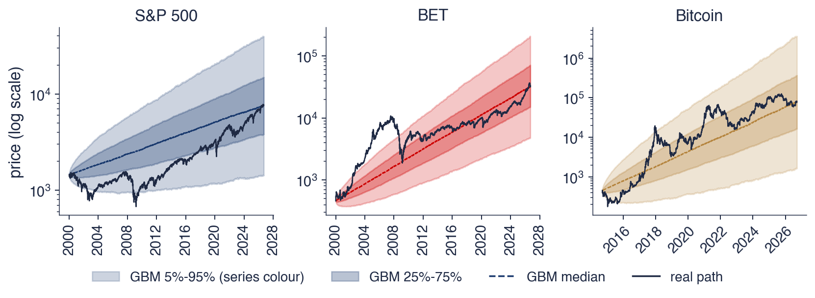
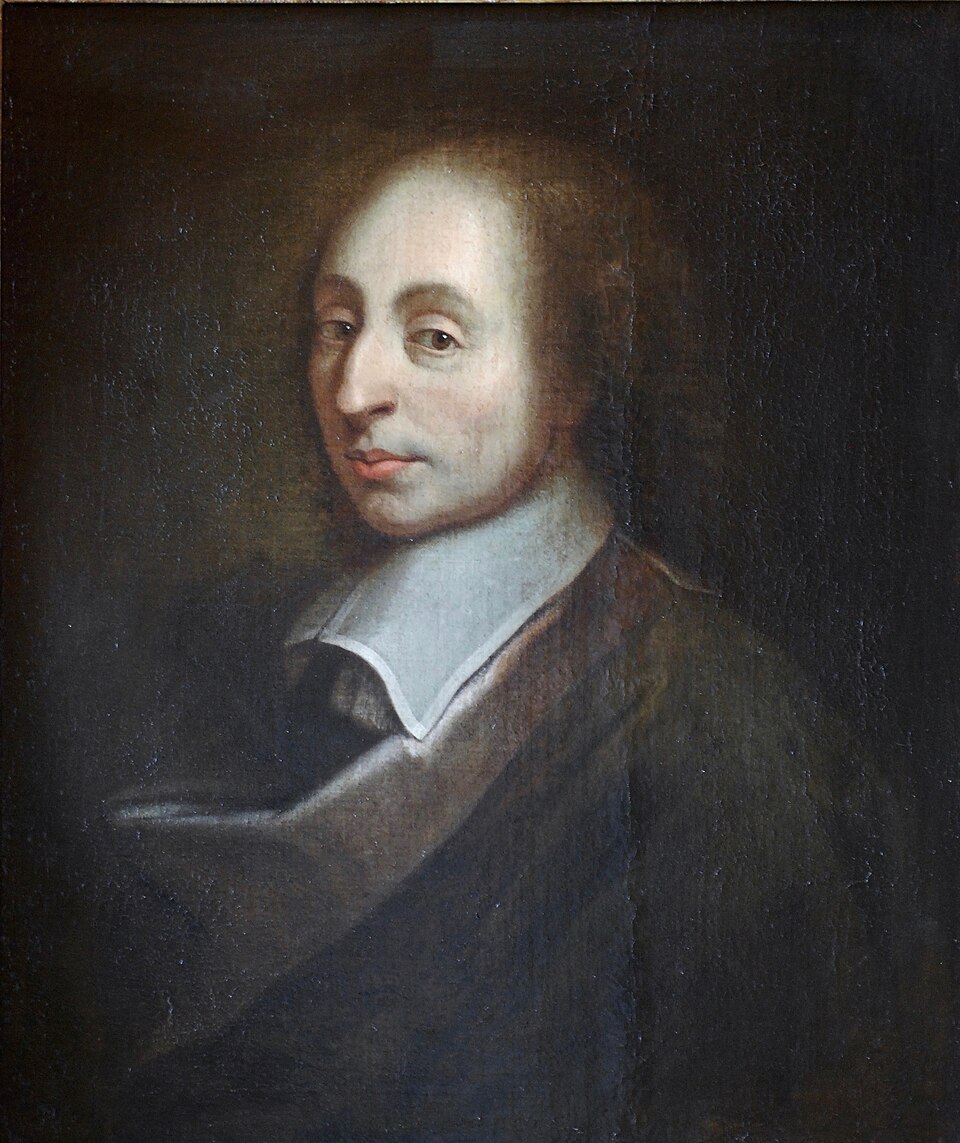
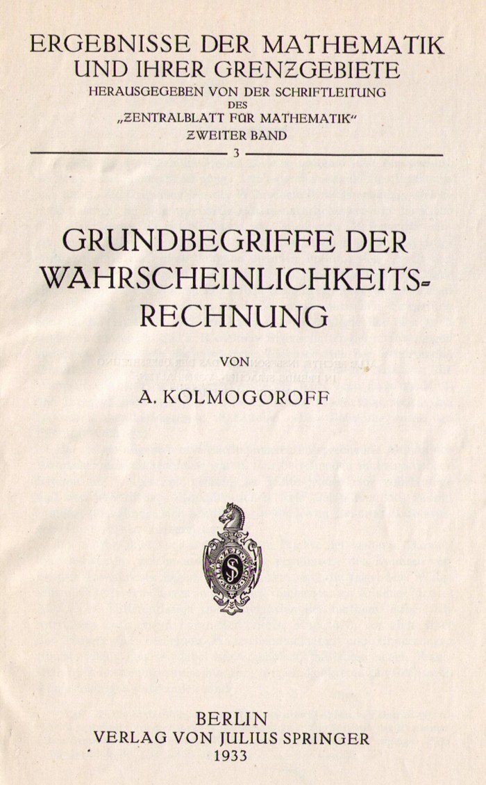

 SFM_ch4_random_variables