Bucharest University of Economic Studies IDA Institute Digital Assets Blockchain Research Center AI4EFin Artificial Intelligence for Energy Finance Romanian Academy, Institute for Economic Forecasting MSCA Digital Finance
“In science, evidence is generated to test hypotheses in an evidence-generating process (EGP). We claim that EGP variation across researchers adds uncertainty—nonstandard errors (NSEs).” — Menkveld et al. (2024)
Menkveld et al. (2024): 164 research teams test the same six hypotheses on the same data
for market efficiency, the interquartile range (IQR) of the estimates across teams is 6.7 percentage points (pp)
the median standard error (SE) implies a Gaussian IQR of only 3.4%, half the 6.7 pp
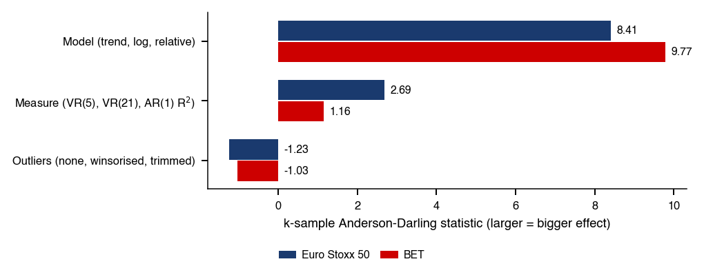
On course data, a mini-multiverse of 27 specifications per index shows the same phenomenon
IQR of the estimated annual trend: 64.6 pp for the Euro Stoxx 50 and 82.6 pp for the BET (Bucharest Exchange Trading), the benchmark index of the Bucharest Stock Exchange
benchmark due to sampling alone: 41.3 pp and 43.4 pp, respectively
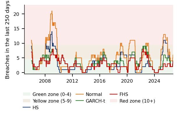
The choice of risk model also changes the conclusion: VaR 1% (Value-at-Risk) for the BET over 5 432 evaluation days
the Normal model is breached on 2.25% of days, more than twice as often as it should
only FHS (filtered historical simulation), at 1.23%, lies in the 95% binomial range [0.74%, 1.27%]
The chapter reviews Chapters 0–18 through seven pitfalls and prepares the team project
replication, pre-registration and a specification grid
In science, evidence is generated to test hypotheses in an evidence-generating process (EGP). We claim that EGP variation across researchers adds uncertainty—nonstandard errors (NSEs).
The chapter asks when an empirical result about markets deserves trust, and when it only reflects the data, the design or luck. In the experiment of Menkveld et al. (2024), 164 research teams test the same six hypotheses on the same data: all trades in Euro Stoxx 50 index futures from 2002–2018, 720 million records. For market efficiency, the median estimate is −1.1% per year and the interquartile range (IQR) of the estimates across teams is 6.7 percentage points (pp). The median standard error (SE) of 2.5% implies a Gaussian IQR of 3.4%, half the 6.7 pp: the dispersion across teams is twice the one that sampling alone would produce.
The same phenomenon appears on course data. A mini-multiverse combines three decisions, the treatment of outliers, the inefficiency measure and the model, into 27 specifications per index, applied to daily closes from 2002–2018. The IQR of the estimated annual trend is 64.6 pp for the Euro Stoxx 50 and 82.6 pp for the BET, the Bucharest Stock Exchange index, above the benchmark due to sampling alone, 41.3 pp and 43.4 pp, respectively. The choice of model drives the dispersion: for the nine specifications with a linear trend, the IQR is only 2.6 pp and 6.7 pp, respectively.
The first part of the chapter reviews Chapters 0–18 through six pitfalls and an integrated case study, from raw BET prices to a backtested 1% Value-at-Risk (VaR). Over the 5 432 evaluation days, the Normal model is breached on 2.25% of days, more than twice as often as it should, and only filtered historical simulation (FHS), at 1.23%, lies in the 95% binomial range [0.74%, 1.27%]. The second part prepares the team project: replication, pre-registration, the specification grid and the declared use of AI (Artificial Intelligence).
AppendixThe project guide, derivations and full tables.
Criteria for an Empirical Finding
The last regular chapter turns from new methods to the question that every earlier chapter raised in passing: when is an empirical result about markets a finding, and when is it an artefact of the data, the design or chance. It reviews Chapters 0–18 under that question, isolates six pitfalls that recur across them and runs one integrated case study, before the second part prepares the team project.
An estimate becomes a finding only when it survives the questions that could explain it away: whether it reflects the particular data set, a design choice made after seeing the data, or luck among many attempts. The chapter treats this question as its subject rather than as a footnote to a method.
Part I gives the course in one picture, reviews Chapters 0–18 and isolates six pitfalls, then follows one integrated case study from raw prices of the BET, the benchmark index of the Bucharest Stock Exchange (BVB), to a backtested value-at-risk (VaR) at 1%. The main thread is the one built in the volatility and risk chapters: GARCH (generalised autoregressive conditional heteroskedasticity) forecasts volatility, DCC (dynamic conditional correlation) the correlations, and VaR and ES (expected shortfall, the mean loss beyond VaR) turn them into a loss. Part II covers the team project, the use of artificial intelligence (AI) in the project, a research case study on nonstandard errors and the AI discovery loop; the project is described step by step in the Appendix.
In brief
The Chapter in Brief
The question: when does an empirical result about markets deserve trust?
and when does it only reflect the data, the design or luck?
Part I: the course in one picture, a review of Chapters 0–18
seven pitfalls
one integrated case study, from raw prices of the BET to a backtested value-at-risk (VaR) at 1%
BET: the benchmark index of the Bucharest Stock Exchange, BVB
The main thread: GARCH forecasts volatility, DCC the correlations, VaR and ES turn them into a loss
To compute a backtested risk forecast from the data, with valid inference.
To interpret an empirical result after checking the six pitfalls in one's own code.
To compute the power of the main test of a project, within a plan that includes replication, identification and a specification grid.
The Further Topics, after the Conclusions, and the Appendix contain detailed examples and advanced topics and are reading for familiarity.
In brief
What you should be able to do
Compute a backtested risk forecast from the data, with valid inference
Interpret an empirical result after checking the seven pitfalls in your own code
Compute the power of the main test within a project plan with replication, identification and a specification grid
Further Topics and Appendix: reading for familiarity
Detailed examples and advanced topics are in Further Topics, after the Conclusions
the footer button leads there; the Back button returns to the starting slide
Structure of the Course
The section places the eighteen chapters on one map and states the questions that any model of the course has to answer. The map shows which chapters build on which; the questions turn the map into a checklist for the project.
The diagram arranges the chapters in four rows: markets and pricing (Chapters 0–4), volatility and risk (5–8), high frequency and continuous time (9–12), and learning and new markets (13–18). The arrows mark which chapter feeds which, and the red boxes and arrows mark the main thread of the course.
The red path runs from stylised facts to risk forecasts that can be tested. Chapter 1 establishes heavy tails, volatility clustering and almost no linear predictability of returns. Chapters 5–8 build on these facts: GARCH gives the conditional volatility \(\sigma_{t+1}\), VaR and ES turn it into a loss, and backtesting says whether the forecast can be trusted.
The other rows refine or extend the thread. Chapters 9–12 measure volatility better, with intraday data, and model it in continuous time, with option prices and the VIX, the implied-volatility index of the S&P 500 (Standard & Poor's). Chapters 13–15 bring flexible models, including large language models (LLMs), which are judged with the evaluation tools of Chapter 8. Chapters 16–18 apply the same toolkit to crypto-assets, bubbles and the financial system as a whole, and the special Chapter 20 forecasts realised volatility with path signatures on the VOLARE data (VOLatility Archive for Realized Estimates). Further inference formulas, for the Shanken correction, quasi-maximum likelihood (QMLE) and the empirical quantile, are in the Appendix.
In brief
Red: the main thread, from stylised facts to risk forecasts we can test
Chapter 1: heavy tails, volatility clustering, almost no linear predictability
Chapters 5–8: GARCH gives \(\sigma_{t+1}\), VaR and ES the loss
backtesting says whether to trust it
Chapters 9–12 measure volatility better and model it in continuous time
intraday data, option prices, the VIX
VIX: the implied-volatility index of the Standard & Poor's 500 index (S&P 500)
Chapters 13–15 bring flexible models, including large language models (LLMs)
Five questions apply to every model of the course:
For the data: which series, which calendar and which adjustments, for dividends, splits and holidays.
For the model: which stylised fact it captures and which it ignores.
For estimation: on which window, and with which information available at time \(t\).
For evaluation: whether the forecast is judged out of sample, with a loss that matches the target, such as QLIKE (the quasi-likelihood loss) for a variance or FZ0 (the Fissler–Ziegel score) for a (VaR, ES) pair.
For uncertainty: whether the result comes with robust standard errors, a bootstrap and a test against a simple benchmark.
If one answer is missing, the result is not yet a finding.
In brief
Before estimating
Data: which series, which calendar, which adjustments (dividends, splits, holidays)?
Model
which stylised fact does it capture?
which stylised fact does it ignore?
Estimation: on which window, with which information at time \(t\)?
After estimating
Evaluation: out of sample, with a loss that matches the target?
QLIKE (the quasi-likelihood loss) for variance
FZ0 (the Fissler–Ziegel score) for a (VaR, ES) pair
Uncertainty: robust standard errors, bootstrap, a test against a simple benchmark?
If one answer is missing, the result is not yet a finding
Review of Chapters 0–18
Each slide of the review gives the central result of one chapter together with the formula behind its inference and the condition under which that inference holds. A recurrent condition is a finite fourth moment of returns, which Chapter 1 questions; the review flags it wherever it applies.
Chapter 0 describes markets that combine exchanges, over-the-counter dealers, funds such as exchange-traded funds (ETFs), algorithms and blockchains. From 2015 to 2026, SPY, the S&P 500 ETF with dividends reinvested, had a compound annual growth rate (CAGR) of 13.7% and an annualised volatility of 17.6%; Bitcoin, over the same period, a CAGR of 60.6% and a volatility of 66.7%. The BET lost 82.5% from July 2007 to February 2009.
For i.i.d. log returns, with \(Y\) the sample length in years, \(T\) the number of daily returns and \(K\) the population kurtosis, the standard errors of the annualised mean and of the volatility are
The second formula requires a finite fourth moment. For SPY, \(\mathrm{SE}(\hat\mu_{\text{ann}}) \approx 5.1\%\) for an annualised mean log return of 12.8%: means are barely estimable, while volatilities are.
In brief
Markets combine exchanges, over-the-counter dealers, funds, algorithms and blockchains
Chapter 1 shows that returns are uncorrelated but not independent (Cont, 2001): their magnitude is predictable, their sign largely is not. The tail index \(\alpha\) describes how fast the probability of a loss above \(x\) decays, like \(x^{-\alpha}\). The Hill estimator (Hill, 1975) uses the \(k\) largest losses, ordered \(L_{(1)} \ge \dots \ge L_{(k+1)}\):
For the BET, with \(k = 153\),\(\hat\alpha = 2.39\), with a block-bootstrap 95% confidence interval (CI) of [2.12, 3.03]. The i.i.d. interval \(\hat\alpha \pm 1.96\,\hat\alpha/\sqrt{k} = [2.01, 2.77]\) is narrower, because large losses come in clusters. With \(\alpha < 4\) the fourth moment is likely infinite. Days beyond \(5\sigma\) are more than 1,000 times more frequent than under the Normal distribution, which gives \(2\Phi(-5) \approx 5.7 \times 10^{-7}\) a day, one such day in about 7,000 years.
In brief
Returns are uncorrelated but not independent Cont (2001)
their magnitude is predictable, their sign largely is not
Tail index \(\alpha\): the probability of a loss above \(x\) decays like \(x^{-\alpha}\)
The Hill estimator uses the \(k\) largest losses, ordered \(L_{(1)} \ge \dots \ge L_{(k+1)}\)Hill (1975)
The efficient market hypothesis states that prices fully reflect the information set, and any test of abnormal-return predictability is a joint test of efficiency and of the expected-return model (Fama, 1970). The variance ratio over \(q\) periods and its heteroskedasticity-robust statistic (Lo & MacKinlay, 1988) are
and \(z^*(q)\) requires a finite fourth moment. Several horizons are tested at once with \(\max_q |z^*(q)|\) and the critical values of Chow & Denning (1993).
The share of rolling windows that reject the random walk is 6.7% for the S&P 500, 22.4% for the BET and 0.0% for Bitcoin. A statistical rejection is not an exploitable profit.
In brief
The efficient market hypothesis: prices fully reflect the information set
A test of abnormal-return predictability is a joint test Fama (1970)
of efficiency and of the expected-return model
The \(q\)-period variance ratio and its heteroskedasticity-robust statistic Lo & MacKinlay (1988)
Factor models state that expected returns reward only exposure to systematic factors. The GRS (Gibbons–Ross–Shanken, test) test (Gibbons, Ross & Shanken, 1989) that all intercepts, the pricing errors \(\hat\alpha\), are zero uses \(T\) periods, \(N\) assets and \(K\) factors:
where \(\hat\mu_f\) are the factor means and \(\hat\Sigma\),\(\hat\Omega\) the residual and factor covariance matrices. The \(F\) distribution is exact only under i.i.d. Normal errors.
On 25 size and book-to-market portfolios, the slope of the security market line (SML) is −4.4%, and GRS is 4.18, against a 5% critical value below 1.6, so the capital asset pricing model (CAPM) is rejected (\(p < 0.01\)). Among sector ETFs, the first principal component, the market, explains 66% of the variance.
In brief
Expected returns should reward only exposure to systematic factors
The GRS (Gibbons–Ross–Shanken) test that all intercepts (pricing errors) \(\hat\alpha\) are zero Gibbons, Ross & Shanken (1989)
\(T\) periods, \(N\) assets and \(K\) factors
\begin{equation*} \mathrm{GRS} = \frac{T - N - K}{N}\,\frac{\hat\alpha^\top\hat\Sigma^{-1}\hat\alpha}{1 + \hat\mu_f^\top\hat\Omega^{-1}\hat\mu_f} \;\sim\; F(N, T - N - K) \end{equation*}
\(\hat\mu_f\): factor means; \(\hat\Sigma\), \(\hat\Omega\): residual and factor covariances
the \(F\) is exact only under i.i.d. Normal errors
25 size and book-to-market portfolios
SML (security market line) slope \(-4.4\%\)
GRS \(= 4.18\), against a 5% critical value below 1.6
the CAPM (capital asset pricing model) is rejected (\(p < 0.01\))
Sector ETFs: the first principal component (the market) explains 66% of the variance
Markowitz (1952) asks the right question, but estimation error dominates the answer. For i.i.d. Normal returns over \(T\) periods, the standard error of the per-period Sharpe ratio (Lo, 2002) is
which again requires a finite fourth moment. In samples of 60 months, the median in-sample Sharpe ratio is 1.56 while the median true Sharpe ratio is only 0.30, and 96% of the estimated tangency portfolios are truly worse than the equal-weight rule 1/N (DeMiguel, Garlappi & Uppal, 2009), a hard benchmark.
A portfolio A is compared with 1/N by testing \(SR_A - SR_B = 0\) with HAC (Heteroskedasticity and Autocorrelation Consistent, standard errors) or studentised bootstrap inference (Ledoit & Wolf, 2008), not by comparing two point estimates.
In brief
Markowitz asks the right question, but estimation error dominates the answer Markowitz (1952)
Standard error of the per-period Sharpe ratio, i.i.d. Normal returns over \(T\) periods Lo (2002)
Portfolio A against 1/N: test \(SR_A - SR_B = 0\) with HAC (heteroskedasticity- and autocorrelation-consistent) standard errors or studentised bootstrap inference Ledoit & Wolf (2008)
Volatility clusters, so today's shock predicts tomorrow's variance (Engle, 1982). With \(\varepsilon_t\) the shock and \(\alpha\),\(\beta\) the weights of the last shock and of the last variance, the GARCH(1,1) model of Bollerslev (1986) and its \(h\)-day forecast are
with the long-run level \(\bar\sigma^2 = \omega/(1-\alpha-\beta)\).
The persistence \(\alpha + \beta\) is the rate at which the forecast returns to \(\bar\sigma^2\), and the half-life is \(h_{1/2} = \ln 0.5/\ln(\alpha+\beta)\). For the S&P 500, 2000–2026, \(\alpha + \beta = 0.9948\), so \(h_{1/2} = 132\) days. For the BET the persistence cannot be bounded away from 1, which is the subject of the pitfall on persistence near 1.
Correlations move with the macro regime, so diversification is not guaranteed. In a crisis the measured correlation rises mechanically with volatility, so the test is run on the adjusted correlation of Forbes & Rigobon (2002),
where \(\rho\) is the crisis correlation and \(\delta\) the relative rise in the variance of the source market from calm to crisis; the test on \(\rho^*\) requires a finite fourth moment.
The correlation between SPY and TLT, the long US (United States) Treasury bond ETF, rose from −0.40 to 0.11 after 2022, and over the same time the volatility of a 60/40 portfolio went from 10.4% to 13.2%. The DCC correlation between Bitcoin and SPY was 0.04 before 2020 and 0.31 since.
In brief
Correlations move with the macro regime
diversification is not guaranteed
Crisis correlation rises mechanically with volatility, so test on the adjusted correlation Forbes & Rigobon (2002)
VaR is a quantile of the loss, and ES, the average loss beyond it, is a coherent risk measure. With \(q_\alpha\) the \(\alpha\)-quantile of the returns \(r\) and a continuous distribution,
For the daily S&P 500, the historical VaR 1% is 3.45% and the ES 1% is 5.03%, while the Normal distribution gives a VaR 1% of only 2.80%: heavy tails matter. Filtered historical simulation and conditional extreme value theory (EVT) react to volatility within days (McNeil & Frey, 2000).
In brief
VaR is a quantile of the loss
ES, the average loss beyond it, is coherent
Definitions, with \(q_\alpha\) the \(\alpha\)-quantile of the returns \(r\) (continuous distribution)
A VaR forecast is backtested on the number and the timing of its breaches, with the coverage test of Kupiec (1995) and the independence test of Christoffersen (1998). With \(x\) breaches in \(T\) days and the observed rate \(\hat\pi = x/T\), the Kupiec statistic is
The Christoffersen statistic \(LR_{ind} \sim \chi^2_1\) compares the breach rate after a quiet day with the rate after a breach; its formula is given in Step 4 of the case study.
For the S&P 500, VaR 1%, 2007–2026, the breach rates against a target of 1% are 2.70% for the Normal model, 1.67% for historical simulation (HS), 1.23% for filtered historical simulation (FHS) and 1.15% for GARCH-EVT, a GARCH filter with a tail from extreme value theory. On the S&P 500 and the BET, a GARCH filter combined with a flexible tail wins: FHS and GARCH-EVT.
Intraday prices measure daily variance as realised variance, \(RV\). The log-HAR (heterogeneous autoregressive) model of Corsi (2009) approximates its observed persistence over finite horizons:
with \(\overline{\ln RV}^{(5)}_t\) and \(\overline{\ln RV}^{(22)}_t\) the means of \(\ln RV\) over the last 5 and 22 days. A stationary HAR (Heterogeneous AutoRegressive, model) is a finite autoregression and therefore has short memory asymptotically.
For SPY, the kurtosis of open-to-close returns is 15.73, and 2.66 after dividing by \(\sqrt{RV_t}\). Log-HAR beats GARCH(1,1)-\(t\) in QLIKE by 10% for SPY (\(p = 0.021\)) and by 22% for Bitcoin. The Diebold–Mariano (DM) test on QLIKE requires finite moments and weak dependence of the loss differential \(d_t\), not of the returns.
Prices form in limit order books, and the bid–ask spread pays for order processing, inventory and adverse selection. The bid–ask bounce makes consecutive changes of the transaction price, \(\Delta p_t\), negatively correlated, which gives the Roll spread
When the sample covariance is positive the estimator is undefined, and how often this happens must be reported.
The Amihud illiquidity ratio, in basis points (bp) per 1 million US dollars (USD), is 0.0016 for SPY, 24.7 for Banca Transilvania and 1,024.0 for Transelectrica. For SPY, the opening five-minute bar moves 2.06 times as much as a midday bar.
In brief
Prices form in limit order books
The spread pays for processing, inventory and adverse selection
The Roll spread: the bid–ask bounce
makes consecutive changes of the transaction price, \(\Delta p_t\), negatively correlated
Brownian motion is the limit of random walks with ever smaller steps, and Itô's lemma solves the stochastic differential equations of prices. Geometric Brownian motion (GBM) implies Normal log returns, which the Jarque–Bera test checks with the sample skewness \(S\) and kurtosis \(K\):
For the S&P 500 there are 62 days beyond ±4 standard deviations, against 0.59 expected under GBM, and the Hill index of S&P 500 losses is below 4 (Chapters 1 and 16), so the fourth moment is likely infinite. Jumps are detected with the standardised difference between realised variance and bipower variation \(BV\), which is robust to jumps and converges to \(N(0,1)\)(Barndorff-Nielsen & Shephard, 2006).
In brief
Brownian motion is the limit of random walks with ever smaller steps
Itô’s lemma solves the stochastic differential equations of prices
Normality of the log returns of geometric Brownian motion (GBM)
the Jarque–Bera test, with \(S\) the sample skewness and \(K\) the sample kurtosis
Black & Scholes (1973) price options by hedging. Implied volatility, the value of \(\sigma\) extracted from option prices, is a risk-neutral quantity, not a forecast of physical volatility. The ex-ante variance risk premium is \(E_t^Q[RV_{t,t+21}] - E_t^P[RV_{t,t+21}]\), where \(RV_{t,t+21}\) is the realised variance over the next 21 trading days; \(VIX_t^2\) estimates the first term, while the second needs a forecast.
The ex-post realised gap, \(VIX_t^2 - RV_{t,t+21}\), is known only at \(t+21\), and consecutive values overlap, so its mean needs Newey–West standard errors with at least 21 lags and a finite fourth moment. Over 1990–2026 the mean VIX is 19.4 and the mean realised volatility over the next month 15.3. The gap is positive on 86% of days, but not in crashes, and its sign does not identify the sign of the ex-ante premium.
Machine learning brings flexible models to data with little signal and much noise (López de Prado, 2018), so the finance-specific part is the validation process. Shuffled K-fold cross-validation reports 69.4% accuracy on pure noise, because of leakage, test information that leaks into training. The remedy is purging, which drops training labels that overlap the test fold, and an embargo after the test fold.
When one strategy is selected among \(N\), the deflated Sharpe ratio of Bailey & López de Prado (2014) tests \(SR > \mathbb{E}[\max_N \widehat{SR}]\), the expected best estimated Sharpe ratio of \(N\) no-skill strategies, a threshold that grows with \(N\). For fractional differencing of the S&P 500, a unit-root test with one lag rejects from \(d^* = 0.25\); the rejection does not prove stationarity, because the finite filter's weights sum to a nonzero value (0.178 at \(d = 0.25\)), and the correlation of 0.98 with the log price only illustrates the component that remains. No model beats the naive rule "always up".
the finance-specific part is the validation process
Shuffled K-fold reports 69.4% accuracy on pure noise
leakage: test information leaking into training
Remedy: purging and an embargo after the test fold
purging: dropping training labels that overlap the test fold
Selection among \(N\) strategies: the deflated Sharpe ratio tests \(SR > \E[\max_N \widehat{SR}]\)Bailey & López de Prado (2014)
the threshold: the expected best estimated Sharpe ratio of \(N\) no-skill strategies
the threshold grows with \(N\)
S&P 500, fractional differencing of order \(d\): a unit-root test with one lag rejects from \(d^* = 0.25\)
a rejection by the ADF (Augmented Dickey–Fuller) test does not prove stationarity: the finite filter has weights summing to a nonzero value (\(0.178\) at \(d = 0.25\)), so the series keeps a component proportional to the log price
its correlation with the log price, \(0.98\), only illustrates this component
No model beats the naive rule “always up”
Chapter 14: Deep Learning and Time-Series Foundation Models
LSTMs (long short-term memory networks) and Transformers learn from sequences, and foundation models forecast zero-shot, without training on the series at hand. Two models are compared with the Diebold–Mariano test (Diebold & Mariano, 1995) on the loss differences \(d_t\),
where \(\hat\Omega\) is the heteroskedasticity and autocorrelation consistent (HAC) long-run variance of \(d_t\).
For SPY realised volatility, QLIKE (lower is better) is 0.223 for Chronos-2, 0.226 for log-HAR and 0.273 for GARCH-\(t\), on the exact grid of 78 five-minute bars; Chronos-2 and log-HAR are not significantly different (DM \(p = 0.539\)). The VaR 1% of Chronos-2 without recalibration has 1.67% breaches on the S&P 500. With many candidate models, the model confidence set (MCS) of Hansen, Lunde & Nason (2011) replaces pairwise tests.
In brief
LSTMs (long short-term memory networks) and Transformers learn from sequences
Foundation models forecast zero-shot
without training on the series at hand
The Diebold–Mariano test on loss differences \(d_t\) between two models Diebold & Mariano (1995)
\(\hat\Omega\): the HAC long-run variance of \(d_t\)
From dictionaries to FinBERT and LLMs, text becomes a number. The predictive regression \(r_{t+1} = a + b\,S_t + \varepsilon_{t+1}\), with \(S_t\) the sentiment score, has a known problem (Stambaugh, 1999): a persistent \(S_t\) whose innovations correlate with returns biases \(\hat b\) and its \(t\)-test.
Classifiers scored on the same texts are compared as pairs, with the exact McNemar test. On financial headlines, Qwen 7B is more accurate than Qwen 1.5B by 21.5 percentage points (McNemar \(p < 0.001\)). A headline-sentiment strategy has a Sharpe ratio of +0.63 before costs and −1.48 after costs, with a break-even cost of 1.5 bp per trade.
In brief
From dictionaries to FinBERT and LLMs: text becomes a number
Predictive regression \(r_{t+1} = a + b\,S_t + \varepsilon_{t+1}\), \(S_t\) the sentiment score Stambaugh (1999)
a persistent \(S_t\) whose innovations correlate with returns biases \(\hat b\) and its \(t\)-test
Classifiers scored on the same texts are compared as pairs, with the exact McNemar test
Qwen 7B vs 1.5B on financial headlines: \(+21.5\) percentage points in accuracy
McNemar \(p < 0.001\)
A headline-sentiment strategy: Sharpe \(+0.63\) before costs
The case study of Chapter 16 (Pele et al., 2023) shows that cryptocurrencies form a distinct asset class in a feature space where a tail factor separates them, and decentralised finance (DeFi) runs on smart contracts. For the link between Bitcoin and the S&P 500, the sup-Wald statistic of Andrews (1993), the largest Wald statistic over candidate break dates, is 20.1, against a 5% critical value of 11.6. The Wald statistic requires \(\mathbb{E}[x_t^2u_t^2] < \infty\), a fourth-order condition on regressor and error. The estimated break is 9 March 2020, not the 2024 launch of spot ETFs.
The Hill tail index of losses is 2.73 for Bitcoin, 95% CI [2.12, 3.33], and 2.87 for the S&P 500, 95% CI [2.07, 3.67]. The difference between them, from a joint block bootstrap, is −0.14 with a 95% CI of [−1.68, 0.71]. The interval contains 0, so there is no evidence of heavier Bitcoin tails; a non-rejection is not equality, and the overlap of the two separate intervals is not a test of the difference.
In brief
The chapter case study (Pele et al. (2023)): cryptocurrencies form a distinct asset class
in a feature space where a tail factor separates them
DeFi (decentralised finance) runs on smart contracts
A bubble is a price path that grows faster than fundamentals can justify. GSADF, the largest right-tailed ADF (augmented Dickey–Fuller) statistic over all sample fractions \([r_1, r_2]\) of length at least \(r_0\)(Phillips, Shi & Yu, 2015), is
Shifts in volatility distort its size, so wild-bootstrap critical values are used. For weekly Bitcoin, 2014–2026, GSADF is 3.85, against a 95% wild-bootstrap critical value of 2.82 (2.27 by Monte Carlo), so explosive episodes are detected. The test of one against two Markov regimes for Bitcoin gives a likelihood ratio (LR) of 123.2, against a parametric-bootstrap 95% critical value of 11.8 (\(p = 0.005\)).
In brief
A bubble is a price path that grows faster than fundamentals can justify
Systemic risk is the risk that losses of one institution spread to the whole system. \(\Delta\)CoVaR (Conditional Value-at-Risk of the system given an institution in distress) measures the change in the system's VaR when institution \(i\), with return \(X^i\), moves from its median to distress:
For the \(\Delta\)CoVaR 1% of eleven banks, 4 of the 25 within-region pairs differ at 5%, and none after the Holm correction; comparing the overlap of intervals alone would have ranked none.
LRMES, the expected loss of a bank when the market falls by more than 10% over 22 days, is simulated from GJR (Glosten–Jagannathan–Runkle, asymmetric GARCH)–GARCH and DCC models (Brownlees & Engle, 2017). For JPMorgan it is 10.6% today and was 23.7% with the information of 31 March 2020.
In brief
Systemic risk: losses of one institution that spread to the whole system
\(\Delta\)CoVaR: the change in the system’s VaR when institution \(i\) moves from its median to distress
\(\Delta\)CoVaR 1% of eleven banks: 4 of 25 within-region pairs differ at 5%
0 after the Holm correction
Overlap of intervals alone would have ranked none
LRMES, simulated from GJR–GARCH (Glosten–Jagannathan–Runkle asymmetric GARCH) and DCC Brownlees & Engle (2017)
LRMES: the expected loss of a bank when the market falls by more than \(10\%\) over 22 days
JPMorgan \(10.6\%\) today, \(23.7\%\) with the information of 31 March 2020
Section summary
The chapter results share a structure: an estimate, a formula for its uncertainty and an assumption under which that formula holds. The fourth-moment condition recurs across variance ratios, Sharpe ratios, correlation tests and Wald statistics, and it is exactly the condition that the tail estimates of Chapter 1 put in doubt.
Common Methodological Errors
The review shows the same mistakes recurring under different names. The section collects them into six pitfalls, grouped by where they arise: in the design of the study, in the data, in the inference and in the evaluation, with a remedy for each.
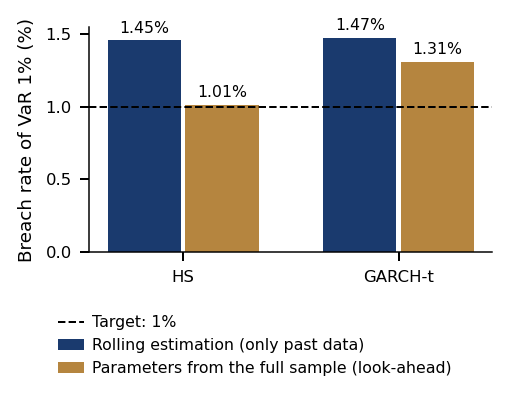
Look-ahead bias arises when a full-sample estimate leaks the future into a forecast: any parameter, threshold or scaling estimated on the whole sample. Examples are full-sample GARCH parameters or standardisation and labels that overlap the test set (Chapter 13); the effect on the BET appears in the case study. The remedy is rolling or expanding windows, purging and an embargo, and the information set \(\mathcal{F}_{t-1}\) written next to every forecast.
Overfitting arises because the in-sample fit rewards noise that will not repeat out of sample (Chapter 4). Backtest overfitting, trying many strategies and keeping the best, is analysed by Bailey et al. (2017), and the deflated Sharpe ratio corrects for the number of trials and for non-normal returns (Bailey & López de Prado, 2014). The remedy is to fix the design before the test period, report every model tried and compare with a simple benchmark: 1/N, historical simulation, the random walk or log-HAR.
In brief
Look-ahead bias: a full-sample estimate leaks the future
any parameter, threshold or scaling estimated on the full sample
Examples: full-sample GARCH parameters or standardisation, labels that overlap the test set (Chapter 13; the effect on the BET: case study)
Remedy: rolling or expanding windows, purging and embargo, the information set \(\mathcal{F}_{t-1}\) written next to every forecast
Overfitting: the in-sample fit rewards noise (Chapter 4)
the noise will not repeat out of sample
Backtest overfitting: trying many strategies and keeping the best Bailey et al. (2017)
In Chapter 3, with 300 useless factors, on average 15.0 pass the threshold \(|t| > 1.96\), and the best reaches \(|t| \approx 3.06\); for this reason the literature asks for \(|t| > 3\)(Harvey, Liu & Zhu, 2016). The same arithmetic applies to calendar anomalies, trading rules and specifications: each extra test adds a chance of a false discovery. The remedy is to count the tests and correct for their number.
In brief
Chapter 3: with 300 useless factors, on average 15.0 pass \(|t| > 1.96\)
With \(m\) tests, ordered p-values \(p_{(1)} \le \dots \le p_{(m)}\) and level \(a\), the three standard corrections reject \(H_{(i)}\) under the following conditions:
\[\begin{array}{ll} \text{Bonferroni:} & p_{(i)} \le a/m, \\ \text{Holm:} & p_{(j)} \le a/(m-j+1) \text{ for every } j \le i, \\ \text{Benjamini–Hochberg:} & i \le \max\{k : p_{(k)} \le k\,a/m\}. \end{array}\]
(19.15)
Bonferroni and the Holm procedure (Holm, 1979) control the probability of any false discovery, the family-wise error rate (FWER), and Holm rejects at least everything Bonferroni rejects. The Benjamini–Hochberg (BH) procedure (Benjamini & Hochberg, 1995) controls the expected share of false discoveries among the rejections, the false discovery rate (FDR). For forecasts, the model confidence set (Hansen, Lunde & Nason, 2011) replaces many pairwise tests.
In brief
With \(m\) tests, ordered \(p\)-values \(p_{(1)} \le \dots \le p_{(m)}\) and level \(a\), reject \(H_{(i)}\) if
\begin{equation*} \begin{array}{ll} \text{Bonferroni:} & p_{(i)} \le a/m \\ \text{Holm:} & p_{(j)} \le a/(m - j + 1) \text{ for every } j \le i \\ \text{Benjamini--Hochberg:} & i \le \max\{k : p_{(k)} \le k\,a/m\} \end{array} \end{equation*}
Bonferroni and Holm Holm (1979) control the chance of any false discovery (FWER)
Holm rejects at least everything Bonferroni rejects
Benjamini–Hochberg (BH) Benjamini & Hochberg (1995) controls the expected share of false discoveries among the rejections (FDR)
Bitcoin trades every day, SPY only on weekdays. The wrong procedure computes each return on its own calendar and then keeps the common days, so Bitcoin's weekend moves disappear. The right procedure keeps the common days of the prices and then computes returns, so that Monday's return covers Friday to Monday for both assets.
The difference is large. For Bitcoin, 2020–2026, on the common days, the cumulative return is 1,025% with the right alignment and 680% with the wrong one, and the standard deviation of Monday returns is 5.04% against 3.83%: the wrong alignment hides weekend risk. The remedy is to align prices on common days first; a series analysed alone stays on its own calendar.
In brief
Bitcoin trades every day, SPY only on weekdays
Wrong: compute each return on its own calendar, then keep the common days: Bitcoin’s weekend moves disappear
Right: keep the common days of the prices, then compute returns: Monday covers Friday to Monday for both
Bitcoin, 2020–2026, on the common days: cumulative return 1 025% (right) against 680% (wrong)
Monday standard deviation 5.04% (right) against 3.83% (wrong): the wrong alignment hides weekend risk
Classical standard errors assume independence and finite moments of the quantity analysed:
For variances, autocorrelations and Sharpe ratios, the fourth moment of returns;
For the DM test, the moments of the loss differential;
For Gaussian QMLE, the fourth moment of the standardised innovations.
For the BET, \(\hat\alpha = 2.39\) with a 95% CI of [2.12, 3.03] (Chapter 1), which under a Pareto-type tail is consistent with an infinite kurtosis, without proving it. The sample excess kurtosis, 11.1, then estimates no finite parameter, and a bootstrap interval for it is not valid (Athreya, 1987); the tail index should be reported instead.
The remedies are HAC standard errors, the block bootstrap where it is valid and intervals that respect the parameter boundary. The Newey–West HAC standard error of a mean \(\bar d\) (Newey & West, 1987) is \(\mathrm{SE}(\bar d) = \sqrt{\hat\Omega/T}\), with
where \(\hat\gamma_j\) is the sample autocovariance at lag \(j\) and \(L\) the number of lags; the Bartlett weights guarantee \(\hat\Omega \ge 0\). The same long-run variance enters the Diebold–Mariano test of Step 5.
In brief
Classical standard errors assume independence and finite moments of the quantity analysed
variances, autocorrelations and Sharpe ratios: the fourth moment of returns; DM: the moments of the loss differential; Gaussian QMLE: the fourth moment of the standardised innovations
BET: \(\hat\alpha = 2.39\), 95% CI \([2.12, 3.03]\) (Chapter 1): under a Pareto-type tail, consistent with an infinite kurtosis, not a proof
The sample excess kurtosis (11.1) estimates no finite parameter if \(\alpha < 4\), and a bootstrap interval for it is not valid Athreya (1987): report the tail index instead
Remedy: HAC errors, block bootstrap, intervals that respect the parameter boundary
block bootstrap where it is valid
The Newey–West HAC standard error of a mean \(\bar d\)Newey & West (1987): \(\mathrm{SE}(\bar d) = \sqrt{\hat\Omega/T}\), with
The restriction \(p = \alpha + \beta \le 1\) on GARCH persistence is a choice, not a property of the model. Its interior gives a finite unconditional variance and a finite half-life, and equality is the IGARCH (integrated GARCH) boundary. Without the restriction, \(p\) slightly above 1 is admissible (Nelson, 1990): the process can still be strictly stationary when \(E\ln(\alpha z_t^2 + \beta) < 0\), but it has no finite variance and no half-life.
For the BET, \(\hat p = 0.9907\) lies inside the region; the difficulty is that the true \(p\) may equal 1. At \(p = 1\) the estimator is not approximately Normal (Andrews, 1999), so the Wald interval [0.974, 1.007] is uninformative under the restriction rather than wrong.
In brief
\(p = \alpha + \beta \le 1\) is a restriction we choose, not a property of GARCH
its interior gives a finite unconditional variance and a finite half-life
equality is the IGARCH (integrated GARCH) boundary
Without it, \(p\) slightly above 1 is admissible Nelson (1990)
the process can still be strictly stationary, when \(E\ln(\alpha z_t^2 + \beta) < 0\)
but it has no finite variance and no half-life
BET: \(\hat p = 0.9907\) is inside the region
the difficulty is the true\(p\), which may equal 1
At \(p = 1\) the estimator is not approximately Normal Andrews (1999)
so the Wald interval [0.974, 1.007] is uninformative under our restriction, rather than “wrong”
The likelihood-ratio test of \(H_0: p = 1\) has the boundary distribution \(\tfrac12\chi^2_0 + \tfrac12\chi^2_1\), whose 5% critical value is 2.71 instead of 3.84. For the BET, \(LR = 1.01\) with a p-value of 0.16, so IGARCH is not rejected. The profile-likelihood CI within \(p \le 1\) is [0.975, 1], so the half-life is at least 27 days, with no finite upper bound.
Boundary critical values apply only when the true parameter can sit on the edge of the parameter space that has been imposed, not whenever an estimate is close to some bound.
In brief
The likelihood-ratio test of \(H_0\colon p = 1\) has the boundary distribution \(\tfrac12\chi^2_0 + \tfrac12\chi^2_1\)
the 5% critical value is 2.71 instead of 3.84
BET: \(LR = 1.01\), \(p\)-value 0.16, so IGARCH is not rejected
Profile-likelihood CI within \(p \le 1\): \([0.975, 1]\)
so the half-life is at least 27 days, with no finite upper bound
Boundary critical values apply only when the true parameter can sit on the edge of the space you imposed
not whenever an estimate is close to some bound
Evaluation Error: a Loss That Cannot Rank the Target
A variance forecast \(f_t\) is compared with a noisy proxy \(\hat\sigma_t^2\), such as \(r_t^2\) or \(RV_t\). The mean squared error (MSE) loss is \((\hat\sigma_t^2 - f_t)^2\) and the QLIKE loss is \(\hat\sigma_t^2/f_t - \ln(\hat\sigma_t^2/f_t) - 1\). With a conditionally unbiased proxy, MSE and QLIKE rank forecasts as the true variance would (Patton, 2011); QLIKE depends only on the ratio of proxy to forecast, so volatile days weigh less than under MSE. In Chapter 9, log-HAR beats GARCH in QLIKE, while the MSE comparison is inconclusive.
ES alone has no strictly consistent scoring function on the usual broad classes of distributions, but the pair (VaR, ES) has one (Fissler & Ziegel, 2016): the FZ0 score used in Step 5, combined with Diebold–Mariano tests. The precision of such comparisons is limited in finite samples (Pele & Mazurencu-Marinescu-Pele, 2026). The remedy is to choose the loss before the comparison and state it in the project report.
In brief
A variance forecast \(f_t\) is compared with a noisy proxy \(\hat\sigma_t^2\) (\(r_t^2\) or \(RV_t\))
the MSE (mean squared error) loss: \((\hat\sigma_t^2 - f_t)^2\)
ES alone has no strictly consistent scoring function (one minimised in expectation only by the correct forecast) on the usual broad classes of distributions
Remedy: choose the loss before the comparison, and state it in the project report
Section summary
Each pitfall has a test that can be run in one's own code:
Recompute with data up to \(t\);
Count the tests;
Align prices before returns;
Report the tail index and HAC errors;
Check whether the true parameter can sit on a boundary;
Fix the loss in advance.
The case study that follows applies these checks to one series.
Integrated Case Study: BET
The case study runs the main thread of the course on one Romanian series, the BET index. It asks one risk question, how much a BET position can lose tomorrow with probability 1%, and answers it in five steps that draw on four chapters: stylised facts, GARCH volatility, VaR forecasts, breach rates, and a formal comparison of the models.
Integrated Case Study: Methods from Four Chapters (1/2)
The question is how much a position in the BET index can lose tomorrow with probability 1%, and which forecast of that loss would have been trusted in real time over 2005–2026. The data are the official daily closing values of the BET from 6 January 2000 to 18 September 2026, 6,670 daily log returns.
The log return in percent is \(r_t = 100\ln(P_t/P_{t-1})\) and the loss is \(L_t = -r_t\). Duplicate records and rows dated on weekends are removed, while days with an unchanged close are kept.
In brief
The question
How much can a BET index position lose tomorrow, with probability 1%?
Which forecast of that loss would we have trusted in real time, 2005–2026?
Data
BET index, official daily closing values, 6 Jan 2000 – 18 Sep 2026
6 670 daily log returns
Log return in %: \(r_t = 100\ln(P_t/P_{t-1})\), loss \(L_t = -r_t\)
Removed: duplicate records and weekend-dated rows
days with an unchanged close kept
Integrated Case Study: Methods from Four Chapters (2/2)
The letter \(\alpha\) has four meanings in the case study:
In Step 1 it is the Hill tail index of losses, 2.39, the rate at which \(P(L > x)\) decays like \(x^{-\alpha}\).
In Step 2 it is the GARCH weight of yesterday's squared shock, 0.192.
In Steps 3–4 it is the VaR level, the promised breach probability of 1%, which enters \(LR_{uc}\) and the dynamic quantile (DQ) test.
In Step 5 it is the ES level of 2.5% used to score the pair (VaR, ES) with the score \(S(v, e; y)\).
Before substituting a number, one must ask which \(\alpha\) the formula means: the Kupiec test needs \(\alpha = 0.01\), never 2.39 or 0.192. The letter \(p\) also has two meanings, the GARCH persistence \(p = \alpha + \beta\) and a p-value.
where \(H_0\) states that the first \(m\) autocorrelations are zero and \(\hat\rho_k\) is the sample autocorrelation at lag \(k\); here \(m = 10\), so the 5% critical value is 18.3.
The next chart has two panels: on the left, the quantiles of the standardised returns against those of the Normal distribution; on the right, the autocorrelation function (ACF) of \(r_t\) and of \(|r_t|\).
In brief
Tails: the Hill tail index \(\hat\alpha\) of losses, with a block-bootstrap 95% CI
Question for the room The Hill tail index of BET losses is 2.39. What does this value say about the kurtosis of the returns?
Answer
For a Pareto-type tail with true index α < 4, the fourth moment is infinite. The Hill estimate of 2.39 and its 95% confidence interval [2.12, 3.03] support this interpretation without proving it. If this tail assumption is correct, the sample excess kurtosis of 11.1 does not estimate a finite parameter; this is why the tail index is reported. The threshold 2 concerns the second moment; the relevant threshold for the fourth moment is 4. Over the full sample, 51 days lie beyond ±4 standard deviations, against 0.42 expected under the Normal distribution.
The left panel compares the quantiles of standardised BET returns with Normal quantiles, so heavy tails appear as points that bend away from the diagonal at both ends. The right panel shows the ACF of returns and of absolute returns, with a band computed for i.i.d. data.
The tails are heavy: the Hill tail index of losses is \(\hat\alpha = 2.39\), with a 95% CI of [2.12, 3.03], so the kurtosis is not reported, since \(\hat\alpha < 4\). There are 51 days beyond ±4 standard deviations, against 0.42 expected under the Normal distribution, and the worst daily loss is −13.1%, on 7 January 2009.
Volatility clusters: the ACF of \(|r_t|\) is 0.40 at lag 1 and decays slowly, and the Ljung–Box statistic \(Q(10)\) on \(r_t^2\) is 2,440, against the critical value 18.3; the usual \(\chi^2\) limit of the test on \(r_t^2\) requires a finite eighth moment. The first-order autocorrelation of the returns, 0.11, is typical of a less liquid market (Chapters 2 and 10). A VaR based on the Normal distribution with constant volatility is therefore too low in stress and too high in calm periods.
In brief
Heavy tails (left)
Hill tail index of losses \(\hat\alpha = 2.39\), 95% CI [2.12, 3.03]
the kurtosis is not reported, because \(\hat\alpha < 4\)
51 days beyond \(\pm 4\) standard deviations, against 0.42 expected under the Normal distribution
worst daily loss \(-13.1\%\), on 7 Jan 2009
Volatility clustering (right)
ACF of \(|r_t|\) at lag 1: 0.40, slow decay (the band assumes i.i.d. returns)
Ljung–Box \(Q(10)\) on \(r_t^2\): 2 440, against the critical value 18.3
the test on \(r_t^2\) requires a finite eighth moment for the usual \(\chi^2\) limit
Step 2 fits a GARCH(1,1) model with Student-\(t\) innovations to the BET daily log returns, 2000–2026, and the chart shows the returns with the band \(\pm 2\hat\sigma_t\). The persistence \(\hat\alpha + \hat\beta\) determines how long a volatility shock lasts, through the half-life of the GARCH review.
Question for the room In GARCH(1,1), the effect of a shock on the variance forecast is carried forward by the factor α + β = 0.9907 per day. After approximately how many days is this effect halved?
Answer
After about 74 trading days: ln 0.5 / ln 0.9907. Using β = 0.799 alone ignores the propagation through future shocks; 1/(1 − p) is not the half-life formula. The persistence cannot be bounded away from 1: the likelihood-ratio test of p = 1 gives LR = 1.01, with p-value 0.16. The profile interval for p, [0.975, 1], maps to a half-life interval with a lower end of about 27 days and no finite upper end.
With robust standard errors, \(\hat\alpha = 0.192\) (0.025), \(\hat\beta = 0.799\) (0.024) and \(\hat\nu = 5.01\) degrees of freedom, so the tails remain heavy even after filtering. The persistence \(\hat\alpha + \hat\beta = 0.9907\) gives a half-life of about 74 trading days, but it cannot be bounded away from 1, as the pitfall on persistence near 1 shows. Daily volatility peaked at 7.39% on 15 October 2008, and at the end of the sample, 18 September 2026, \(\hat\sigma_T = 1.67\%\).
In brief
BET daily log returns with \(\pm 2\hat\sigma_t\) from a GARCH(1,1) with Student-\(t\) innovations, 2000–2026
Step 3 compares two VaR 1% forecasts on the daily BET losses of 2020–2026, with gains set to 0: the Normal VaR estimated on a 500-day window and the FHS VaR, which scales historical standardised returns by the GARCH volatility. The black dots mark losses above the FHS VaR.
Question for the room Over the 1,675 days of 2020–2026, about 17 breaches of the VaR 1% were expected. Which of the two models comes close to this number?
Answer
FHS, with 22 breaches; the Normal model has 41. The FHS VaR rose to 11.6% on 18 Mar 2020, while the Normal VaR, estimated on 500 days, adjusts slowly and its breaches cluster in the first weeks of every stress episode.
FHS reacts within days and peaked at 11.6% on 18 March 2020, during the COVID-19 crash, while the Normal VaR on a 500-day window moves only slowly. Over the 1,675 days of the chart about 17 breaches are expected; FHS has 22 and the Normal model 41, and the Normal breaches cluster in the first weeks of every stress episode. The last VaR forecast is 4.48% for FHS and 2.18% for the Normal model.
In brief
Daily BET losses (gains set to 0), Normal and FHS VaR 1%
black dots: losses above the FHS VaR
FHS reacts within days
it peaked at 11.6% on 18 Mar 2020, during the COVID-19 crash
The Normal VaR on a 500-day window moves only slowly
1 675 days, about 17 breaches expected
FHS 22, Normal 41
Normal breaches cluster in the first weeks of every stress episode
The chart gives, for each of the four models, the share of days with a loss above the VaR 1% forecast over the \(T = 5{,}432\) evaluation days of Step 3. The light-blue band is the 95% binomial range [0.74%, 1.27%] of the observed rate when the true rate is 1%.
Question for the room VaR 1%, 5,432 evaluation days: read separately, the 5% Kupiec tests reject HS, the Normal model and GARCH-t. Does the list of rejected models change if we apply the Holm correction (FWER 5%) to the four tests?
Answer
No. The Kupiec p-values are below 0.001 (Normal, 122 breaches), 0.001 (GARCH-t, 80), 0.002 (HS, 79) and 0.095 (FHS, 67). Holm compares them, in order, with 0.05/4 = 0.0125, 0.05/3 ≈ 0.0167, 0.05/2 = 0.025 and 0.05: the first three pass, FHS does not. The correction makes the tests stricter, so it cannot add rejections. The FHS rate, 1.23%, lies inside the 95% binomial band [0.74%, 1.27%]; the non-rejection does not establish that the true rate is exactly 1%. A rate above 1% does not imply rejection, and numerical closeness to 1% does not replace the test.
Only FHS, at 1.23%, lies inside the band. The Normal model, at 2.25%, breaches more than twice as often as it should.
In brief
Share of days with a loss above the VaR 1% forecast, over the \(T = 5\,432\) evaluation days of Step 3
Light-blue band: the 95% binomial range [0.74%, 1.27%] if the true rate is 1%
Only FHS (1.23%) lies inside the band
the Normal model (2.25%) breaches more than twice as often as it should
The table compares the four models on four criteria:
The dynamic quantile (DQ) test with its p-value;
The average FZ0 score;
The p-value of the model confidence set (MCS);
The zone of a comparative ES backtest.
Only FHS passes the DQ test at 5% (\(p = 0.129\)); GARCH-\(t\) fails it (\(p = 0.007\)) through its excess of breaches.
On the FZ0 score, where lower is better, FHS (1.157) and GARCH-\(t\) (1.175) are not significantly different (DM \(t = 1.39\)), and both beat HS and the Normal model (\(|t| > 4.9\)). The 10% model confidence set is {GARCH-t, FHS}, and the comparative ES backtest puts the Normal model in the red zone and GARCH-\(t\) and FHS in the green zone.
The GARCH-filtered models are superior, and FHS remains the only model rejected by no test of coverage, independence or DQ. The result supports a comparison of procedures; FZ0 scores the pair (VaR 2.5%, ES 2.5%), not the VaR 1% of Steps 3–4.
In brief
Model
\(DQ\)
\(p_{DQ}\)
FZ0
\(p_{MCS}\)
ES zone
HS
192.1
\(<\)0.001
1.422
0.00
standard
Normal
364.6
\(<\)0.001
1.495
0.00
red
GARCH-t
17.9
0.007
1.175
0.18
green
FHS
9.9
0.129
1.157
1.00
green
Only FHS passes the DQ (Dynamic Quantile) test at 5% (\(p = 0.129\))
GARCH-\(t\) fails it (\(p = 0.007\)) through its excess of breaches
FZ0 (lower is better): FHS and GARCH-\(t\) are not significantly different (DM \(t = 1.39\))
both beat HS and Normal (\(|t| > 4.9\))
The 10% model confidence set is {GARCH-t, FHS}
Comparative ES backtest against HS as the standard model: Normal red, GARCH-\(t\) and FHS green
The GARCH-filtered models are superior
FHS remains the only model rejected by no test (coverage, independence, DQ)
Type of evidence: comparison of procedures (it shows which method works better on the same data, not why)
FZ0 scores the (VaR 2.5%, ES 2.5%) pair, not the VaR 1% of Steps 3–4
The question is how often the Kupiec test notices that a VaR 1% model is wrong. At a true breach rate \(\pi\), its power is an exact binomial probability, that of the rejection region \(R_T\) of the 5% test:
At \(\pi = 1\%\) the same sum gives the actual size of the nominal 5% test: 9.48% at \(T = 250\), where \(R_T\) contains 0 breaches and any number from 7 up.
The minimum detectable effect (MDE) is the smallest true rate \(\pi > 1\%\) with \(\text{Power}(\pi) \ge 80\%\). Power grows with \(T\), because the standard error of the observed rate \(\hat\pi\) is \(\sqrt{\pi(1-\pi)/T}\).
In brief
The question: if the VaR 1% model is wrong, how often does the Kupiec test notice?
Power at the true breach rate \(\pi\): an exact binomial probability
the probability of the rejection region \(R_T\) of the 5% test
The chart plots the power (19.18) of the 5% Kupiec test against the true breach rate of a VaR 1% model, for several sample lengths \(T\), from one Basel year of 250 days to the 5,432 days of the case study.
Question for the room Assume independent breaches with a true daily probability of 2% for a VaR 1% model. How does the probability that the 5% Kupiec test rejects the model change when ▶ increases T from 250 to 5,432 days?
Answer
It rises from 24% to almost 100% (78% at T = 1,000). At T = 250 the test rejects at 0 breaches or at 7 or more. The 5% level is nominal and concerns the null; 1 − 5% is not the power either. With the asymptotic critical value 3.84, the actual rejection probability at the null rate of 1% is 9.5% at T = 250. On the page grid, the first true rate detected with at least 80% power is 3.65% at T = 250 (an excess of 2.65 percentage points over the target), 2.05% at T = 1,000 and 1.45% at T = 5,432. A non-rejection with low power means “no evidence”, not “no problem”.
At \(T = 250\), a true breach rate of 2% is detected only 24% of the time. The MDE, searched on a grid with steps of 0.05 percentage points, is 3.65% at \(T = 250\), 2.05% at \(T = 1{,}000\) and 1.45% at \(T = 5{,}432\), and even at \(T = 5{,}432\) a true rate of 1.3% is detected with probability 55% only. A non-rejection with low power means "no evidence", not "no problem", so the power should be stated before the test.
In brief
Exact binomial probability that the 5% Kupiec test rejects a VaR 1% model
by its true breach rate
\(T = 250\) (one Basel year): a true rate of 2% is detected only \(24\%\) of the time
MDE, searched on a grid with steps of 0.05 percentage points
\(3.65\%\) at \(T = 250\), \(2.05\%\) at \(T = 1\,000\), \(1.45\%\) at \(T = 5\,432\)
Even at \(T = 5\,432\), a true 1.3% is detected with probability \(55\%\) only
A non-rejection with low power is “no evidence”, not “no problem”
On the BET, the GARCH filter with historical standardised returns (FHS) is the only VaR 1% forecast that no backtest rejects, while the Normal model breaches more than twice as often as it should. The power calculation shows how much weaker these conclusions would be on one year of data, which is why a project states the power of its main test in advance.
Integrated Case Studies: Portfolio, Bitcoin, Romanian Investor
The BET case study applied five steps to one index. The three studies of this section apply the same logic to three practical decisions: which minimum-variance portfolio and which VaR forecast to hold, which daily loss limit to set for Bitcoin, and whether an investor who counts her wealth in lei should hedge the euro. Each study states its question and its decision rule before the numbers, combines several chapters of the course and ends with what is chosen, under which conditions, and what would make the choice change.
Multi-Asset Portfolio: the Question and the Decision Rule
The first study asks which global minimum-variance (GMV) portfolio of eight exchange-traded funds (ETFs) to hold and which one-day VaR 1% forecast to rely on. The universe is the multi-asset universe of Chapter 4, with daily adjusted prices from April 2007 to July 2026:
Three equity funds (SPY for the US, EFA for developed markets outside the US and EEM for emerging markets);
Two US Treasury funds (TLT, 20+ years, and IEF, 7–10 years);
Two corporate bond funds (LQD, investment grade, and HYG, high yield);
The gold fund GLD (SPDR Gold Shares).
The evaluation runs from 1 May 2012 to 31 July 2026, 3,583 days.
Four chapters supply the steps:
Chapter 4 gives monthly GMV weights from the last 60 months, with the sample covariance or with the shrinkage estimator of Ledoit & Wolf (2004).
Chapter 6 gives the conditional covariance \(H_t\) from GARCH(1,1) and the dynamic conditional correlation (DCC) model of Engle (2002), re-estimated every January.
Chapter 7 gives the portfolio VaR 1% and the Euler risk contributions.
Chapter 8 gives the Kupiec test of coverage and the Christoffersen tests of independence and conditional coverage.
The decision rule is fixed in advance. Up to 2018 the portfolio uses the GMV variant with the lower volatility, and from 2019 the choice is tested out of sample. The VaR forecast must be rejected at 5% by none of the three tests; if several pass, the one with the lower mean VaR is chosen.
In brief
The question: which global minimum-variance (GMV) portfolio of eight ETFs do we hold, and which one-day VaR 1% forecast do we rely on?
The multi-asset universe of Chapter 4, daily adjusted prices, Apr 2007 – Jul 2026
Question for the room Which mechanism can contribute to DCC-FHS (DCC with Filtered Historical Simulation) understating risk, although DCC-FHS and DCC-Normal use the same conditional covariance?
Answer
The FHS history reuses the data on which the GMV weights were optimised, which can make the historical risk too small: the mean standard deviation of the standardised portfolio returns across the FHS windows is 0.91, while the standard deviation of the out-of-sample standardised returns is 0.95. FHS multiplies the empirical quantile of the standardised losses by the current volatility: the mean VaR is 0.55%, against 0.58% for DCC-Normal. DCC-FHS has 52 breaches against 35.8 expected (Kupiec p 0.011); DCC-Normal has 40 breaches and passes all three tests. These results support the diagnosis without isolating the contribution of each mechanism. The comparison is retrospective: the VaR model is chosen on the same period on which it is evaluated.
The chart combines the three steps of the study: the rolling one-year volatility of the two GMV portfolios, the daily VaR 1% forecasts with their breaches, and the Euler shares of the four asset classes in the portfolio risk. The numbers are on the next slide.
The portfolio step compares the two covariance estimates out of sample. The GMV portfolio with the sample covariance has an annualised daily volatility of 4.13%, the Ledoit–Wolf version 4.28%, with a mean shrinkage intensity \(\delta = 0.17\). Shrinkage buys stability: monthly turnover is 0.085 against 0.135, and the gross exposure of the target weights, \(\sum_i |w_i|\), has a mean of 1.80 against 2.42 and a maximum of 2.30 against 3.78. Up to 2018 the volatilities are 3.08% and 3.15%, so the rule picks the sample covariance; from 2019 they are 4.87% and 5.07%.
The risk step forecasts the portfolio volatility \(\sigma_{p,t} = \sqrt{w_t' H_t w_t}\) for day \(t\), with \(w_t\) the weights at the start of the day. At the last re-estimation, January 2026 on 4,712 days, the DCC parameters are \(\hat a = 0.024\) and \(\hat b = 0.968\). Three VaR 1% forecasts are compared:
DCC-Normal, \(2.326\,\sigma_{p,t}\);
DCC with filtered historical simulation (FHS), \(\sigma_{p,t}\) times the 99% quantile of the standardised loss \(-r_{p,s}/\sigma_{p,s}\) over the last 1,000 days;
Historical simulation (HS), the loss quantile over the last 500 days with the weights \(w_t\).
Over the evaluation 35.8 breaches are expected.
The Euler share of asset \(i\) in the variance, \(w_i (H_t w_t)_i / w_t' H_t w_t\), is also its share in VaR and ES (expected shortfall) under an elliptical distribution. On average over the evaluation, Treasuries carry 69% of the risk, credit 17%, equities 12% and gold 2%. On 27 March 2020, the day with the highest \(\sigma_{p,t}\) (0.98%), credit carries 63% of the risk with a weight of 25%.
In brief
(a) Chapter 4: daily out-of-sample volatility, annualised (in the chart: over a rolling year)
GMV with the sample covariance: 4.13% a year
GMV with Ledoit–Wolf shrinkage: 4.28% a year, with a mean shrinkage intensity \(\delta = 0.17\)
monthly turnover: 0.085 with Ledoit–Wolf, against 0.135
gross exposure \(\sum_i |w_i|\) of the target weights: mean 1.80 with Ledoit–Wolf, against 2.42; maximum 2.30, against 3.78
to 2018: 3.08% against 3.15%: the rule picks the sample covariance; from 2019: 4.87% against 5.07%, so the choice holds
(b) Chapters 6–8: \(\sigma_{p,t} = \sqrt{w_t' H_t w_t}\), the forecast for day \(t\), with \(w_t\) the weights at the start of the day (rebalanced monthly, then drifting with the prices)
DCC at the last re-estimation (Jan 2026, 4 712 days): \(\hat a = 0.024\), \(\hat b = 0.968\)
DCC-Normal: \(\text{VaR} = 2.326\,\sigma_{p,t}\)
DCC-FHS: \(\sigma_{p,t}\) times the 99% quantile of the standardised loss \(-r_{p,s}/\sigma_{p,s}\) over the last 1,000 days
HS: the loss quantile over the last 500 days, with the weights \(w_t\)
35.8 breaches of the VaR 1% expected
(c) Chapter 7: the Euler share \(w_i (H_t w_t)_i / w_t' H_t w_t\) of each asset class in the variance
it is also the share in VaR and ES under an elliptical distribution
mean over the evaluation: Treasuries 69%, credit 17%, equities 12%, gold 2%
27 Mar 2020, the day with the highest \(\sigma_{p,t}\) (0.98%): credit carries 63% of the risk with a weight of 25%
Multi-Asset Portfolio: the Result and the Decision
The table reports, for the three VaR 1% forecasts, the number and rate of breaches, the p-values of the Kupiec, independence and conditional-coverage tests, and the mean VaR. Only DCC-Normal passes all three tests: 40 breaches (1.12%), Kupiec \(p = 0.492\), independence \(p = 0.083\), conditional coverage \(p = 0.175\), with a mean VaR of 0.58%. HS fails on independence (48 breaches, independence \(p < 0.001\)), and DCC-FHS fails on coverage and independence (52 breaches, Kupiec \(p = 0.011\)). The DCC-FHS history applies today's weights to the data on which they were estimated, the in-sample understatement of risk of Chapter 4: the standard deviation of \(r_{p,s}/\sigma_{p,s}\) is 0.91 inside the FHS window and 0.95 outside it.
The result supports a retrospective comparison of procedures, on one portfolio and one period, and the VaR model is chosen on the same period on which it is evaluated. The independence p-value of DCC-Normal, 0.083, is below 10%; the minimum detectable effect (MDE) of the Kupiec test at \(T = 3{,}583\) is a breach rate of 1.55%, and no transaction costs are included.
The choice is the GMV portfolio with the sample covariance and the DCC-Normal VaR 1%, 0.64% for 31 July 2026, under monthly weights and a DCC re-estimated yearly with only the information available on the forecast date. Two results would overturn it:
A rejection of independence on new data;
A gross-exposure limit \(c\), imposed in the optimisation at every rebalancing and checked daily, that the portfolio cannot meet; GMV breaches it for \(c < 3.78\) (3.86 on daily weights), Ledoit–Wolf for \(c < 2.30\) (2.34).
In brief
VaR 1%
Breaches
Rate
Kupiec \(p\)
indep. \(p\)
cond. \(p\)
mean VaR
DCC-Normal
40
1.12%
0.492
0.083
0.175
0.58%
DCC-FHS
52
1.45%
0.011
0.046
0.005
0.55%
HS, 500 days
48
1.34%
0.052
\(<\)0.001
\(<\)0.001
0.63%
Type of evidence: a retrospective comparison of procedures, on one portfolio and one period
only DCC-Normal passes all three tests; the VaR model is chosen on the same period on which it is evaluated
HS fails on independence, DCC-FHS on coverage and on independence
the DCC-FHS history applies today's weights to the data they were estimated on (the in-sample understatement of risk of Chapter 4)
standard deviation of \(r_{p,s}/\sigma_{p,s}\): 0.91 inside the FHS window, 0.95 outside it
Limits
the independence \(p\)-value of DCC-Normal is 0.083, below 10%
the Kupiec MDE at \(T = 3\,583\): 1.55%; no transaction costs
What I choose: GMV with the sample covariance and the DCC-Normal VaR 1% (0.64% for 31 Jul 2026)
Under which conditions: monthly weights and DCC re-estimated yearly, with only the information available on the forecast date
What would make me drop it
a rejection of independence on new data
a gross-exposure limit \(c\): imposed in the optimisation at every rebalancing and checked daily; GMV breaches it for \(c < 3.78\) (daily: 3.86), Ledoit–Wolf for \(c < 2.30\) (2.34)
The second study takes the view of a risk manager who holds Bitcoin: which one-day loss limit should she set, and which signal would make her cut the position? The data are daily closes from 18 September 2014 to 18 September 2026, 4,384 returns, and 5-minute bars on UTC (Coordinated Universal Time) days from 1 September 2024 to 17 September 2026, 659 complete days.
Five chapters supply the tools:
The stylised facts of Chapter 1;
Realised variance RV and the log-HAR forecasts of Corsi (2009) from Chapter 9;
The backtests of the VaR 1% from Chapter 8;
Spreads and Amihud illiquidity from Chapter 10;
The GSADF bubble test with BSADF (Backward Sup Augmented Dickey–Fuller, statistic) date-stamping of Phillips, Shi & Yu (2015) from Chapter 17.
The daily limit is the log-HAR VaR 1% if it is not rejected at 5% and needs less capital on average than HS; otherwise it is the HS VaR, which is also used on days without a log-HAR forecast because the 5-minute bars are incomplete. The position is cut when BSADF stays above its 95% wild-bootstrap critical value for at least 7 weeks in a row, the minimum episode length \(\lceil \ln T \rceil = 7\) weeks of Chapter 17.
In brief
The question: a risk manager holds Bitcoin; which one-day loss limit does she set, and which signal would make her cut the position?
Question for the room The evaluation has 422 days. How often would the 5% Kupiec test reject a VaR 1% model whose true breach rate is 2%?
Answer
Only with probability 47%; the minimum detectable effect at 80% power is 2.70%. Both models have 7 breaches against 4.2 expected (p = 0.214), so the practical difference is capital: a mean VaR of 5.29% for log-HAR, against 6.24% for HS.
The chart shows the three inputs of the Bitcoin decision: the BSADF statistic against its wild-bootstrap critical value, the log-HAR and HS VaR 1% forecasts with their breaches, and the Amihud illiquidity of Bitcoin and SPY.
The daily returns show the stylised facts of Chapter 1 in strong form. The Hill tail index of losses is 2.71 (\(k = 109\), 2.5% of the days), annualised volatility is 66.6%, the autocorrelation of \(|r_t|\) at lag 1 is 0.21, and 29 days lie beyond ±4 standard deviations, against 0.28 expected under the Normal distribution.
The log-HAR model regresses \(\ln RV\) on its 1-, 7- and 30-day means, with \(R^2 = 0.36\) and coefficients \(\hat\beta_d = 0.38\) (Newey–West standard error 0.04), \(\hat\beta_w = 0.47\) (0.08) and \(\hat\beta_m = -0.02\) (0.10). Expanding-window forecasts start on 1 March 2025 and cover 422 days, as in Chapter 9. The VaR 1% is \(2.326\sqrt{\widehat{RV}_t}\), with a mean of 5.29% and a range from 1.99% to 14.45%, against a mean of 6.24% for HS on the last 500 days. Of the 566 calendar days, 144 have no log-HAR forecast, so the evaluation covers days selected by data availability. The standardised return \(r_t/\sqrt{\widehat{RV}_t}\) has a standard deviation of 1.00, an excess kurtosis of 2.54 and a 1% quantile of −2.52, against −2.33 for the Normal distribution.
Liquidity is not a constraint. The Amihud illiquidity, in basis points (bp) per USD 1 million traded, is 0.0037 for Bitcoin over the last two years, against 0.0016 for SPY; its monthly mean fell from 0.80 over the first 12 months from 2016 to 0.0040 over the last 12. Spreads estimated from daily data disagree: 85 bp for Roll, 81 bp for Corwin–Schultz and −8 bp for EDGE (Efficient Discrete Generalized Estimator). GSADF is 3.85, against a 95% wild-bootstrap critical value of 2.82 (2.27 under homoskedastic Monte Carlo), with explosive episodes in May 2017–January 2018 and December 2020–February 2021. Since 2022 BSADF has exceeded the wild critical value in only 6 weeks, at most 3 in a row (peak 1.47 on 8 March 2024), and its last value is −0.65, against a critical value of 0.58.
expanding-window forecasts from 1 Mar 2025: 422 days, the same as in Chapter 9
(b) Chapter 8: VaR 1% \(= 2.326\sqrt{\widehat{RV}_t}\), against HS on the last 500 days
log-HAR VaR: mean 5.29%, between 1.99% and 14.45%; HS VaR: mean 6.24%
144 of the 566 calendar days have no log-HAR forecast: the evaluation covers the days selected by data availability
\(r_t/\sqrt{\widehat{RV}_t}\): standard deviation 1.00, excess kurtosis 2.54
1% quantile of \(r_t/\sqrt{\widehat{RV}_t}\): \(-\)2.52, against \(-\)2.33 for the Normal distribution
(c) Chapter 10: Amihud illiquidity, in bp per USD 1 million traded
last two years: 0.0037 for Bitcoin, 0.0016 for SPY
monthly mean: 0.80 over the first 12 months from 2016, 0.0040 over the last 12 months
spreads from daily data disagree: Roll 85 bp, Corwin–Schultz 81 bp, EDGE (Efficient Discrete Generalized Estimator) \(-\)8 bp (EDGE estimates the squared spread, which comes out negative when price variance dominates)
(a) Chapter 17: GSADF 3.85, against a 95% wild-bootstrap critical value of 2.82 (homoskedastic Monte Carlo: 2.27)
explosive episodes, with the wild-bootstrap critical values: May 2017 – Jan 2018 and Dec 2020 – Feb 2021
since 2022: BSADF above the wild critical value in 6 weeks, at most 3 in a row (peak 1.47, on 8 Mar 2024)
last value: \(-\)0.65, against a wild critical value of 0.58
On the 422 days with complete bars, from 1 March 2025 to 17 September 2026, both the log-HAR and the HS VaR 1% have 7 breaches against 4.2 expected, with Kupiec \(p = 0.214\), independence \(p = 0.604\) and conditional-coverage \(p = 0.404\). The coverage is the same, and the log-HAR VaR is lower on average by 0.95 percentage points. The independence test uses only the 372 pairs of consecutive calendar days. The full rule, with HS on days without a forecast, has 9 breaches over all 566 days, against 5.7 expected (Kupiec \(p = 0.194\), independence \(p = 0.589\)).
The power is low: the MDE is a breach rate of 2.70%, and a true rate of 2% is detected with probability 47%. Only two years of 5-minute bars are available, the Normal quantile understates the tail (−2.52 against −2.33), and the Amihud measure uses the volume reported by aggregated exchanges. The result supports a retrospective comparison of procedures.
The choice is a daily limit equal to the log-HAR VaR 1%, 5.04% for 17 September 2026, recomputed every day, provided that the 5-minute bars cover at least 95% of the day and illiquidity stays of the order of that of SPY. With 5 or more breaches in 250 days, the Basel yellow zone of Chapter 8, the limit switches to the empirical quantile of \(r_t/\sqrt{\widehat{RV}_t}\). The position is cut when BSADF stays above the wild critical value for 7 weeks in a row; because weekly monitoring repeats the test and a pointwise 95% threshold does not control false alarms over the whole horizon, the signal is confirmed with the family-wise threshold of Chapter 17.
In brief
VaR 1%
Breaches
Expected
Kupiec \(p\)
indep. \(p\)
cond. \(p\)
mean VaR
log-HAR
7
4.2
0.214
0.604
0.404
5.29%
HS, 500 days
7
4.2
0.214
0.604
0.404
6.24%
Type of evidence: a retrospective comparison of procedures, on 422 days with complete bars (1 Mar 2025 – 17 Sep 2026)
the same coverage, with a mean VaR lower by 0.95 percentage points
indep. \(p\): only the 372 pairs of consecutive calendar days
the full rule (HS on days without a forecast), over all 566 days: 9 breaches, against 5.7 expected; Kupiec \(p\) 0.194, indep. \(p\) 0.589
the power is low: MDE 2.70%; a true rate of 2% is detected with probability 47% (power of the Kupiec test)
Limits
only two years of 5-minute bars
the Normal quantile understates the tail: \(-\)2.52, against \(-\)2.33
Amihud uses the volume reported by aggregated exchanges
What I choose: a daily limit equal to the log-HAR VaR 1% (5.04% for 17 Sep 2026), recomputed every day
Under which conditions: the 5-minute bars cover at least 95% of the day; illiquidity stays of the order of that of SPY
What would make me drop it
5 or more breaches in 250 days (the Basel yellow zone, Chapter 8): I switch to the empirical quantile of \(r_t/\sqrt{\widehat{RV}_t}\)
BSADF above the wild critical value for 7 weeks in a row: I cut the position
weekly monitoring repeats the test: a pointwise 95% threshold does not control false alarms over the whole horizon, so I confirm with the family-wise threshold of Chapter 17
A Romanian Investor: the Question and the Decision Rule
The third study takes an investor who measures her wealth in lei and holds 50% in the BET and 50% in the Euro Stoxx 50, bought in euro. The question is whether she should hedge the EUR (euro)/RON currency risk (lei per euro) of the euro leg. The data are daily closes of both indices and the National Bank of Romania (BNR) EUR/RON reference rate, July 2005–September 2026. Exposures and hedging use weekly returns from Friday to Friday, because the BNR fixes the rate at 13:00 and the exchanges close at different times.
The minimum-variance hedge ratio \(h^*\) over a rolling three years from Chapter 6;
VaR 1% and ES 2.5% by historical simulation from Chapter 7.
The benchmark is the result of Campbell, Serfaty-de Medeiros & Viceira (2010): a currency that is negatively correlated with equities lowers risk, so a full hedge does not minimise risk. Three choices are compared, with \(h\) the share of the euro leg sold forward: no hedge (\(h = 0\)), the rolling \(h^*\), and a full hedge (\(h = 1\)). The rule picks the choice with the lowest weekly ES 2.5%; if the ES values differ by less than 0.25 percentage points in every period, it picks \(h = 0\), which needs no forward contracts.
In brief
The question: an investor who measures her wealth in lei holds 50% BET and 50% Euro Stoxx 50, bought in euro; does she hedge the currency risk of the euro leg, that is, of the EUR/RON rate, the number of Romanian lei (RON) per euro (EUR)?
Data: BET and Euro Stoxx 50 (daily closes), the BNR (Banca Națională a României, the National Bank of Romania) EUR/RON reference rate, Jul 2005 – Sep 2026
weekly (Friday) returns: the BNR fixes the rate at 13:00, the exchanges close at other times
Three choices, with \(h\) the share of the euro leg sold forward: \(h = 0\) (no hedge), rolling \(h^*\), \(h = 1\) (full hedge)
We pick the choice with the lowest weekly ES 2.5%
If the ES values differ by less than 0.25 percentage points in every period: \(h = 0\), which needs no forward contracts; we switch to \(h = 1\) after six months in a row of positive three-year correlation between equities and EUR/RON
A Romanian Investor: Efficiency, Currency Hedging and ES in Lei
Question for the room In the retrospective comparison for Aug 2008 – Sep 2026, which mechanism can explain why a full currency hedge did not lower the ES of the portfolio?
Answer
The negative association between the Euro Stoxx 50 return and the EUR/RON change (β = −0.52, t = −2.61) partly offset the losses: when EUR/RON rises, the leu depreciates and the value in lei of the euro investment rises, other things equal. The association is not a rule that holds every week. The EUR/RON volatility is 4.6% a year, against 20.9% for the Euro Stoxx 50. Weekly ES 2.5%, Aug 2008 – Sep 2026: 9.60% unhedged, 9.67% with a full hedge; in Aug 2008 – Dec 2012 the order reverses (15.23% and 15.12%). This retrospective comparison does not replace the decision rule of the lecture, which chooses the full hedge (h = 1).
The chart shows the inputs of the hedging decision: the rolling three-year correlation between the Euro Stoxx 50 and the change of EUR/RON, the rolling hedge ratio \(h^*\), and the weekly ES 2.5% of the three hedging choices.
Daily returns are tested with the robust variance-ratio statistic \(z^*(q)\), which rejects the random walk at 5% when \(|z^*| > 1.96\). EUR/RON rejects strongly, with \(z^*(2) = 4.76\), VR(2) = 1.17 and a first-order autocorrelation of 0.17; the BET gives \(z^*(2) = 2.08\), but the Chow–Denning joint test over \(q = 2, 5, 10, 20\) gives \(p = 0.067\); the Euro Stoxx 50 has \(|z^*(q)| \le 1.68\) and a Chow–Denning \(p = 0.43\). Because the daily EUR/RON risk multiplied by \(\sqrt{h}\) understates the \(h\)-day risk, the study works on weeks.
The exposures are estimated over 1,101 weeks, with \(f = \Delta\)EUR/RON, so that \(f > 0\) means the leu depreciates. The Euro Stoxx 50 in euro has \(\hat\beta = -0.52\) on \(f\)(\(t = -2.61\)), and the BET has coefficients 0.56 on the Euro Stoxx 50 (\(t = 7.4\)) and −0.54 on \(f\)(\(t = -2.11\)), with \(R^2 = 0.30\): the leu depreciates in the weeks in which equities fall. The GARCH(1,1)-\(t\) models give a EUR/RON persistence of 1.000, at the boundary of stationarity, and current annualised volatilities of 0.96% for EUR/RON (mean 4.4%), 25.9% for the BET (mean 21.2%) and 13.8% for the Euro Stoxx 50 (mean 21.0%).
The minimum-variance hedge ratio is \(h^* = \mathrm{Cov}(r^{RON}, f)/\mathrm{Var}(f)\), with \(r^{RON} = r^{EUR} + f\) the return in lei of the euro leg. On the full sample \(h^* = 0.48\); over a rolling three years it ranges from −4.34 (July 2022) to 1.38 (March 2026), with a last value of 1.27, and the three-year correlation between the Euro Stoxx 50 and \(f\) is negative in 93% of the windows. The weekly ES 2.5% of the 50/50 portfolio, rebalanced weekly, uses the exact simple return
where \(b\) and \(s\) are the log returns of the BET and the Euro Stoxx 50 and the forward is on the notional at the start of the week with zero carry; the loss is \(L = -100\ln(1 + R_p)\) in log points.
In brief
(a) Chapter 2: the robust statistic \(z^*(q)\) on daily returns; \(|z^*| > 1.96\) rejects the random walk at 5%
EUR/RON: \(z^*(2) = 4.76\), with VR(2) \(= 1.17\) and a first-order autocorrelation of 0.17
BET: \(z^*(2) = 2.08\); the Chow–Denning test over \(q = 2, 5, 10, 20\): \(p = 0.067\)
Euro Stoxx 50: \(|z^*(q)| \le 1.68\); Chow–Denning: \(p = 0.43\)
the daily EUR/RON risk times \(\sqrt{h}\) understates the \(h\)-day risk, so we work on weeks
Chapter 3: exposures over 1 101 weeks, with \(f = \Delta\)EUR/RON (\(f > 0\): the leu depreciates)
Euro Stoxx 50 in euro on \(f\): \(\hat\beta = \ensuremath{-}0.52\) (\(t = \ensuremath{-}2.61\))
BET on Euro Stoxx 50 and \(f\): 0.56 (\(t = 7.4\)) and \(-\)0.54 (\(t = \ensuremath{-}2.11\)), \(R^2 = 0.30\)
the leu depreciates in the weeks in which equities fall
EUR/RON: persistence 1.000, at the boundary of stationarity
EUR/RON: volatility today 0.96% a year, against a mean of 4.4%
BET: 25.9% today, against a mean of 21.2%
Euro Stoxx 50: 13.8% today, against a mean of 21.0%
(b) Chapter 6: \(h^* = \mathrm{Cov}(r^{RON}, f)/\mathrm{Var}(f)\), with \(r^{RON} = r^{EUR} + f\) the return in lei of the euro leg
full sample: \(h^* = 0.48\)
over a rolling three years: between \(-\)4.34 (Jul 2022) and 1.38 (Mar 2026); last value 1.27
the three-year correlation between the Euro Stoxx 50 and \(f\) is negative in 93% of the windows
(c) Chapter 7: weekly ES 2.5% of the 50/50 portfolio, rebalanced weekly, for the three choices (table on the next slide)
the exact simple return \(R_p = \tfrac12(e^{b} - 1) + \tfrac12[e^{s + f} - 1 - h(e^{f} - 1)]\), with \(b\), \(s\) the log returns of the BET and the Euro Stoxx 50; a forward on the notional at the start of the week, with zero carry
The table gives the weekly ES 2.5% of the three choices of (19.19) in three periods. Over August 2008–September 2026 (944 weeks) it is 9.60% without a hedge, 9.62% with the rolling \(h^*\) and 9.67% with a full hedge; in 2008–2012 (228 weeks) 15.23%, 15.20% and 15.12%; in 2020–2026 (351 weeks) 8.43%, 8.43% and 8.47%. The ES values differ by at most 0.11 percentage points, so the choice of \(h\) mattered little for the risk. Annualised weekly volatility is 4.6% for EUR/RON and 20.9% for the Euro Stoxx 50, and the negative correlation lets the depreciation of the leu offset part of the losses of the euro leg. The result supports a comparison of hedging choices for one portfolio.
The limits are economic. The cost of the hedge, the RON–EUR interest differential, is not in the course data; the depreciation of the leu added 1.55% a year to the euro leg over July 2005–September 2026, and a forward replaces this with the differential. \(h^*\) is unstable when \(\mathrm{Var}(f)\) is small, as in 2019–2022, the estimation risk of Chapter 4, and it hedges the euro leg only: for the whole portfolio the linear approximation \(\mathrm{Cov}(b + s + f, f)/\mathrm{Var}(f)\) is −0.35.
The current choice is the full hedge, \(h = 1\). The three-year correlation has been positive since 12 September 2025 (0.037 at the end of the sample), which triggered the rule for dropping \(h = 0\) on 13 March 2026, while the rolling \(h^*\) of 1.27 would sell forward more than the euro leg. The choice holds while the three-year correlation between equities and EUR/RON stays positive; a negative correlation for six months in a row would bring the investor back to \(h = 0\).
In brief
Weekly ES 2.5%
Weeks
\(h = 0\)
rolling \(h^*\)
\(h = 1\)
Aug 2008 – Sep 2026
944
9.60%
9.62%
9.67%
Aug 2008 – Dec 2012
228
15.23%
15.20%
15.12%
Jan 2020 – Sep 2026
351
8.43%
8.43%
8.47%
The retrospective conclusion: the ES values of the three choices differ by at most 0.11 percentage points, so the choice of \(h\) mattered little for the risk
annualised weekly volatility: EUR/RON 4.6%, Euro Stoxx 50 20.9%
the negative correlation lets the depreciation of the leu offset part of the losses of the euro leg
Type of evidence: comparison of hedging choices, for one portfolio
Limits
the cost of the hedge, the RON–EUR interest differential, is not in the course data
the depreciation of the leu added 1.55% a year to the euro leg (Jul 2005 – Sep 2026); a forward replaces it with that differential
\(h^*\) is unstable when \(\mathrm{Var}(f)\) is small, as in 2019–2022: the estimation risk of Chapter 4
\(h^*\) hedges the euro leg; for the whole portfolio, \(\mathrm{Cov}(b + s + f, f)/\mathrm{Var}(f) = \ensuremath{-}0.35\) (linear approximation)
What I choose now: the full hedge (\(h = 1\))
the three-year correlation is positive after 12 Sep 2025 (0.037 at the end): the rule for dropping \(h = 0\) was triggered on 13 Mar 2026
the rolling \(h^*\) (1.27) would sell forward more than the euro leg
Under which conditions: the three-year correlation between equities and EUR/RON stays positive
What would make me drop it: a negative three-year correlation for six months in a row (back to \(h = 0\))
Section summary
The three studies follow the same template: a question, a decision rule fixed in advance, steps from several chapters, and a decision with its conditions and its exit rule. In each the evidence is a retrospective comparison of procedures on one portfolio or asset, and in each the limits, low power, short samples or missing costs, are stated next to the decision.
The Team Project
The project is where the course methods are applied to one question chosen by the team. This section gives its four steps, the replication standard, how to choose a question, the grading criteria and the timeline.
The project is an empirical study of one question about financial markets, answered with the methods of this course. It counts for 70% of the final grade; quizzes and seminar activity count for 20% and attendance for 10%.
It has four steps:
The team replicates one full table or figure of a published paper, or of the lecture, cell by cell.
The team extends the analysis with new data, a new market such as the Bucharest Stock Exchange (BVB) or crypto, or a more recent sample, under a pre-analysis plan recorded in a dated commit before the test period is opened; the plan states the null, the test, the loss, the sample split, the identification strategy, the power of the main test and the specification grid with its correction.
The team delivers a GitHub repository that regenerates every number, with the files `AI_USE.md` and `AI_ERRORS.md`.
The team presents the work as a team and defends it orally for 10 minutes: each member explains one result and answers a "what changes if…" question, and grades can differ between members.
In brief
An empirical study of one question about financial markets, answered with the methods of this course
70% of the final grade
quizzes and seminar activity 20%, attendance 10%, no final exam
1. Replicate: one full table or figure of a published paper (or of the lecture)
cell by cell (standard: next slide)
2. Extend: new data, a new market (the BVB, crypto) or a more recent sample
under a pre-analysis plan recorded in a dated commit before the test period is opened
The plan states the null, the test, the loss, the sample split, the identification strategy, the power of the main test and the specification grid with its correction
3. Deliver on GitHub: a repository that regenerates every number
The replication target is one full table or figure, identified by its DOI, page and table number, not a single coefficient. The report compares the published and the team's values cell by cell, gives the difference and explains each gap by sample, filter, data vendor or definition.
Large-scale replications show why this standard matters: many anomalies shrink out of sample or with better data (Hou, Xue & Zhang, 2020), while most factors replicate once the design is right (Jensen, Kelly & Pedersen, 2023). Reproducibility requires a lockfile of package versions, fixed random seeds, the names and dates of the data series, and one command that regenerates every number. Different teams working on the same data disagree more than their standard errors suggest (Menkveld et al., 2024), and more reproducible work is associated with a smaller gap, as the case study of this chapter shows.
In brief
Target: one full table or figure, with its DOI (Digital Object Identifier), page and table number, not a single coefficient
Report a cell-by-cell comparison: published value, your value, difference, and the reason for each gap (sample, filter, data vendor, definition)
Feasible (data that can be obtained and cleaned in a few weeks, such as the course data sets in the course GitHub repository, BNR rates, Federal Reserve Economic Data (FRED), the Kenneth French Data Library or DefiLlama);
Relevant (the answer matters to an investor, a bank or a regulator).
The slide's examples show how a question is narrowed. "Is Bitcoin risky?" is too vague; "Did spot ETFs change the one-day VaR 1% of Bitcoin?" is better, and "Which model forecasts it best since 2024?" can follow. "Can machine learning predict the market?" is too broad; "Does a boosting model beat log-HAR for next-day BET volatility, in QLIKE, 2018–2026?" is a project.
In brief
A good question is
Specific: one market, one period, one quantity
Testable: a null hypothesis and a benchmark
Feasible: data you can obtain and clean in a few weeks
the course data sets in the course GitHub repository
the National Bank of Romania, BNR; Federal Reserve Economic Data, FRED; Kenneth French Data Library; DefiLlama
Relevant: an answer matters to an investor, a bank or a regulator
Examples
Too vague: “Is Bitcoin risky?”
Better: “Did spot ETFs change the one-day VaR 1% of Bitcoin?”
Then: “Which model forecasts it best since 2024?”
Too broad: “Can machine learning predict the market?”
Better: “Does a boosting model beat log-HAR for next-day BET volatility, in QLIKE, 2018–2026?”
In the first week after this chapter the team forms, chooses its question and writes a one-page proposal (Seminar 19, C2), and opens the GitHub repository. Weeks 2–3 cover the data and the replication, and the extension plan is recorded in a dated commit. Weeks 4–5 cover the extension, the evaluation and the robustness checks. In the final weeks the team writes the 8–12-page report, completes the repository with a README and the two AI files, and presents and defends the work. Exact dates are announced at the course and the seminar.
In brief
Week 1 after this chapter: team, question, one-page proposal
AI assistants are allowed for code, debugging, literature search and writing. Their use must be declared, since undeclared use of AI counts as plagiarism, and it is checked: the team is responsible for every line, and a reference that does not exist counts as fabricated data. No AI is used during the oral defence, where "the AI wrote it" is not an explanation.
Two files document the use:
`AI_USE.md` lists the tools and versions, who used them for what, where AI-written code or text was kept, and how the team verified the replicated table, the data, the formulas and the references.
`AI_ERRORS.md` records at least three places where the assistant was wrong: what was asked, what it answered, what was wrong, how the team found out and the correct version.
Errors caught are a strength of the project, not a weakness.
In brief
Policy
Allowed: AI assistants for code, debugging, literature search and writing
Declared: undeclared use of AI counts as plagiarism
Checked: you are responsible for every line
a reference that does not exist counts as fabricated data
No AI during the oral defence: “the AI wrote it” is not an explanation
The case study measures how much the conclusions of empirical finance depend on the researcher rather than on the data. It summarises a crowd-sourced study in which many teams tested the same hypotheses on the same data, then repeats its logic on the course data with a small grid of analysis paths.
In Menkveld et al. (2024), published in the Journal of Finance 79(3) as the Finance Crowd Analysis Project (#fincap), 164 research teams test the same six hypotheses on the same data. The usual standard error measures the uncertainty from sampling, the data-generating process. The nonstandard error measures the uncertainty from the analysis path that each researcher picks, the evidence-generating process.
In the paper's model, team \(j\) reports \(X_j = e_j + \varepsilon_j\), where \(e_j\) is the researcher fixed effect of its path and \(\varepsilon_j\) the sampling error. The nonstandard error is the interquartile range (IQR) of the estimates across teams,
\[\mathrm{NSE} := Q_{0.75}(x) - Q_{0.25}(x),\]
(19.20)
where \(Q_p(x)\) is the \(p\)-quantile of the team estimates \(x\). The IQR is used rather than the standard deviation because the \(e_j\) can have fat tails.
In brief
Menkveld et al. (2024): 164 research teams test the same six hypotheses on the same data
Journal of Finance 79(3)
Finance Crowd Analysis Project, #fincap
Standard error
Uncertainty from sampling, the data-generating process
Nonstandard error: uncertainty from the analysis path each researcher picks, the evidence-generating process
Model: team \(j\) reports \(X_j = e_j + \varepsilon_j\), \(e_j\) the researcher fixed effect of its path, \(\varepsilon_j\) the sampling error
Nonstandard error \(:= Q_{0.75}(x) - Q_{0.25}(x)\), the interquartile range (IQR) of the estimates across teams, \(Q_p(x)\) being the \(p\)-quantile of the team estimates \(x\)
The IQR, not the standard deviation, because the \(e_j\) can have fat tails
The data are all trades in the Euro Stoxx 50 index futures from 2002 to 2018, 720 million records. The six hypotheses each state that there is no annual trend in a market quantity, such as market efficiency, the realised spread or the client share of volume, and each team reports the average yearly change in percent with its standard error (SE). The study ran in four stages in 2021: independent analysis, peer feedback, sharing of the five best papers, and final estimates; the design details are in the Appendix.
The link with this chapter is direct. Every team project is one path through the "garden of forking paths", and pre-registration, the specification grid and a repository that reruns every number are the remedies the course asks for.
In brief
Data
All trades in the Euro Stoxx 50 index futures, 2002–2018, 720 million records
Six hypotheses of “no annual trend” (market efficiency, realised spread, client share of volume, ...)
Each team reports the average yearly change in % with its standard error (SE)
Four stages in 2021: independent analysis, peer feedback, the five best papers shared, final estimates
The dispersion is large. For market efficiency the median estimate is −1.1% per year, with an IQR (19.20) of 6.7 percentage points (pp); even for the client share of volume, a simple ratio, the IQR is 1.2 pp around −3.3% (Table I, Panel C). The median SE of 2.5% would imply a Gaussian IQR of \(1.35 \times 2.5 = 3.4\%\), half the observed 6.7 pp, and the null of no dispersion is rejected for all six hypotheses with \(p < 0.0001\) (Table II).
Quality matters but does not remove the dispersion (Table III, Fig. 2). A rise of one standard deviation in reproducibility is associated with a 25.0% lower IQR, and the same rise in peer rating with a 33.3% lower IQR; code that reruns end to end goes with answers closer to the consensus. The result supports a description of the dispersion across teams; the link with quality is only an association.
In brief
Size
For market efficiency the median estimate is \(-1.1\%\) per year, with an IQR of 6.7 percentage points (pp)
Even for the client share of volume, a simple ratio, the IQR is 1.2 pp around \(-3.3\%\) (Table I, Panel C)
The median SE of 2.5% implies a Gaussian IQR of \(1.35 \times 2.5 = 3.4\%\), half the 6.7 pp
The no-dispersion null is rejected for all six hypotheses, \(p < 0.0001\) (Table II)
Quality (Table III, Fig. 2)
a rise of one standard deviation in reproducibility is associated with a 25.0% lower IQR
the same rise in peer rating, with a 33.3% lower IQR
Code that reruns end to end is associated with answers closer to the consensus
Type of evidence: description (it shows what happened in the data, without testing a cause)
of the dispersion across teams; the link with quality is only an association
The course repeats the logic on daily closes from 2002 to 2018, without the artificial fills on non-trading days (the rule of Chapter 2). The grid crosses three forks, outliers, measure and model, into 27 analysis paths, and the band reported is the IQR across them, the nonstandard error of this multiverse.
The measures of inefficiency are departures from a random walk: \(|VR(q) - 1|\), where \(VR(q)\) is the variance ratio of Chapter 2 with the Lo–MacKinlay corrections at \(q = 5\) and 21 days, and the \(R^2\) of a first-order autoregressive AR(1) model. A positive trend in these measures means declining efficiency.
In brief
Daily closes 2002–2018 from the course data, without the artificial non-trading-day fills (the rule of Chapter 2)
The band is the IQR, the nonstandard error of the multiverse
Measures of inefficiency
\(|VR(q) - 1|\) (\(VR(q)\): the variance ratio of Chapter 2, with the Lo–MacKinlay corrections, \(q = 5, 21\) days) and the \(R^2\) of an autoregressive AR(1) model: departures from a random walk
Question for the room Over all 27 paths, the IQR of the Euro Stoxx 50 estimates is 64.6 pp. ▶ restricts the grid, in turn, to a single model of the yearly change. What does the IQR of the nine linear-trend paths become?
Answer
About 2.6 pp (BET: 6.7 pp, against 82.6 pp over the full grid). With relative differences, the medians are +98.7% and +80.3% a year: the model of the yearly change separates the distributions of the estimates the most. The sampling benchmark, 1.35 × the median SE, is 41.3 pp over the full grid and 3.9 pp for the nine linear-trend paths. The comparison is descriptive, not an estimate of the share of dispersion due to each choice.
The chart shows, for the Euro Stoxx 50 and the BET, the 27 trend estimates of the multiverse sorted from lowest to highest, with the IQR band; the legend defines \(VR(q)\), AR(1), IQR and pp.
In brief
Legend: \(VR(q)\), the \(q\)-day variance ratio; AR(1), the first-order autoregressive model; IQR, the interquartile range; pp, percentage points. MFM_ch19_nonstandard_errors
The IQR of the estimates is 64.6 pp for the Euro Stoxx 50 and 82.6 pp for the BET, around medians of −0.3% and −3.7% a year. The model fork creates the dispersion: over the nine linear-trend paths the IQR is only 2.6 pp for the Euro Stoxx 50 and 6.7 pp for the BET, while relative differences explode, with medians of +98.7% and +80.3% and values up to 48,415%.
The sampling benchmark is the Gaussian IQR, 1.35 times the median SE: 41.3 pp for the Euro Stoxx 50 and 43.4 pp for the BET. The multiverse IQR exceeds it for both indices. The result supports a description of the dispersion over the 27 paths of the grid, not across real teams.
In brief
IQR of the estimates: 64.6 pp (Euro Stoxx 50) and 82.6 pp (BET)
around medians of \(-0.3\%\) and \(-3.7\%\) a year
The model fork creates the dispersion
Over the nine linear-trend paths the IQR is only 2.6 pp for the Euro Stoxx 50 and 6.7 pp for the BET
Relative differences explode: medians \(+98.7\%\) (Euro Stoxx 50) and \(+80.3\%\) (BET), up to \(48\,415\%\)
Sampling benchmark: the Gaussian IQR, \(1.35 \times\) the median SE
\(41.3\) pp (Euro Stoxx 50) and \(43.4\) pp (BET)
The IQR exceeds this benchmark for both indices
Type of evidence: description
of the dispersion over the 27 paths of the grid, not across real teams
Their multiverse covers only a few forks and explains the reported estimates poorly;
Beliefs about dispersion were elicited as standard deviations rather than IQRs;
The test of dispersion assumes consistent reported SEs.
The course replication adds two:
A multiverse spans only the options in its grid, so its IQR neither estimates nor bounds from below the dispersion across real teams.
With daily closes only, the paper's intraday frequency pairs cannot be run.
The open extension asks whether a pre-registered grid shrinks the nonstandard error of a risk question, by measuring the IQR of VaR 1% conclusions for the BET across defensible paths.
In brief
Authors: the multiverse covers a few forks only and explains the reported estimates poorly
Authors: beliefs were asked as standard deviations, not IQRs
Authors: the test of dispersion assumes consistent reported SEs
Our replication: a multiverse spans only the options in its grid
so its IQR neither estimates nor bounds from below the dispersion across real teams
Our replication: daily closes only
so the paper’s intraday frequency pairs cannot be run
Open extension: does a pre-registered grid shrink the nonstandard error of a risk question?
Measure the IQR of VaR 1% conclusions for the BET across defensible paths
AI for Scientific Discovery
The section applies the AI-assisted research loop to the team project itself: how much of a result comes from the data and how much from the researcher, how the loop and its checks fit the project calendar, and one replication and extension worked on the course results.
The open question is how much of a result is the data and how much the researcher. Replication is not hopeless: in a Bayesian model of replication, most asset-pricing factors replicate and work out of sample in 93 countries (Jensen, Kelly & Pedersen, 2023). AI assistants make every extra specification almost free, so the forking paths multiply, but so does the ability to report all of them.
In formal terms, the conclusion must hold over a pre-registered set \(\mathcal{S}\) of defensible specifications, with the family corrected for the family-wise error rate (FWER) or the false discovery rate (FDR). The report gives the distribution of the result over \(\mathcal{S}\), not the best cell.
In brief
Open question: how much of a result is the data, and how much the researcher?
Replication is not hopeless: in a Bayesian model of replication most asset-pricing factors replicate and work out of sample in 93 countries Jensen, Kelly & Pedersen (2023)
AI assistants make every extra specification almost free: the forking paths multiply, but so does the ability to report all of them
Formal version: the conclusion must hold over a pre-registered set \(\mathcal{S}\) of defensible specifications, with the family corrected (FWER or FDR)
Report its distribution over \(\mathcal{S}\), not the best cell
The loop follows the project calendar. In week 1 the team states the question with \(H_0\) and \(H_1\); in weeks 1–2 it reviews the literature and fixes a replication target seen in the PDF of the paper; in week 2 it pre-registers the extension in a dated commit before the first extension result. In weeks 2–3 the replication becomes a passing test in the repository, in weeks 4–5 the whole grid is run, and before the defence an AI examiner questions the team.
In brief
Loop
Question and \(H_0\)/\(H_1\) (week 1)
Literature and the replication target seen in the PDF (weeks 1–2)
Pre-registration of the extension, recorded in a dated commit before the first extension result (week 2)
Replication as a passing test in the repository (weeks 2–3)
The replication target is the FHS VaR 1% for the BET. Chapter 8 reports 59 breaches in 4,937 days (1.20%, Kupiec \(p = 0.181\)); the case study of this chapter finds 67 in 5,432 days (1.23%, \(p = 0.095\)). The model is the same, but the evaluation starts in 2007 in one case and in 2005 in the other, with different settings, so every gap must be documented before a replication is called failed.
A typical assistant proposal reads: "only GARCH-EVT is correctly calibrated on both markets". The assistant reads each p-value alone at 5%, which ignores that the tests form a family.
In brief
Replicate: FHS VaR 1% for the BET
Chapter 8 reports 59 breaches in 4 937 days (\(1.20\%\), Kupiec \(p = 0.181\))
The case study of this chapter: 67 in 5 432 days (\(1.23\%\), \(p = 0.095\))
Same model, different evaluation start (2007 vs 2005) and settings: document every gap before calling a replication failed
A typical assistant proposal: “only GARCH-EVT is correctly calibrated on both markets”
The extension treats the 12 conditional-coverage tests of Chapter 8, for the S&P 500 and the BET and six models each, as one family; Bitcoin and EUR/RON stay outside it because some GARCH forecasts are missing on these markets. At 5% there are 8 rejections without correction, 6 with the Holm correction (FWER) and 7 with the Benjamini–Hochberg (BH) procedure at an FDR of 5%.
FHS fails only on the S&P 500 (\(p = 0.040\)), and within the family of 12 this rejection is no longer significant, so after Holm both FHS and GARCH-EVT pass on both markets. The statement "FHS fails for the S&P 500" therefore depends on whether the test is read alone or in its family. The result supports a comparison of procedures; in the project the family is fixed in the plan before the results are seen, and both readings are reported.
In brief
Extend
The 12 conditional-coverage tests of Chapter 8 (S&P 500 and BET \(\times\) 6 models) form one family
Bitcoin and EUR/RON stay outside the family: on these markets some GARCH forecasts are missing (Chapter 8)
Rejections at 5%: 8 without correction, 6 with Holm (FWER), 7 with Benjamini–Hochberg, BH (FDR 5%)
FHS fails only on the S&P 500 (\(p = 0.040\)); within the family of 12 this rejection is no longer significant, so after Holm FHS and GARCH-EVT pass on both markets
Interpretation: “FHS fails for the S&P 500” depends on whether the test is read alone or in its family
Type of evidence: comparison of procedures
In the project, fix the family in the plan before seeing results and report both readings
The capstone plan starts from the team's project idea from Part C of the seminars, written as \(H_0\) and \(H_1\) together with the observation that would falsify it. The team first replicates one published table seen in the paper and turns it into a passing test in the repository, then extends the analysis over a pre-registered grid with the family corrected and the full distribution reported.
The deliverables follow the timeline: proposal, replication target and pre-registration commit; passing replication test and grid of results; mock defence, report and oral defence. The AI log keeps the prompts that changed the design in `AI_USE.md` and every caught error, with the test that caught it, in `AI_ERRORS.md`; templates are in the project folder.
In brief
Question: your project idea from Part C, written as \(H_0\)/\(H_1\), with the observation that would falsify it
Replicate first: one published table seen in the paper, turned into a passing test in the repository
Then extend over a pre-registered grid, with the family corrected and the full distribution reported
Deliverables along the timeline
proposal and replication target, pre-registration commit
Returns are hard to predict, but their risk is not: volatility, tails and dependence can be forecast. Every model is judged out of sample, against a simple benchmark and with a loss that fits the target. Heavy tails change inference, so robust errors and the bootstrap replace textbook formulas, intervals are reported and power is stated.
Most wrong results come from the design, not from the model: look-ahead, overfitting, multiple testing and misaligned calendars. The analysis path is itself a source of uncertainty, which is why the course asks for pre-registration, replication and a report of the whole grid. New tools, machine learning (ML), foundation models and large language models (LLMs), raise the bar for evaluation rather than lower it.
In brief
Returns are hard to predict, their risk is not
volatility, tails and dependence can be forecast
Every model is judged out of sample, against a simple benchmark, with a loss that fits the target
Heavy tails change inference
use robust errors and the bootstrap
report intervals, state the power
Most wrong results come from the design, not from the model
below the 5% critical value of 3.84, so the model is not rejected. At \(T = 400\) the test has little power, so the outcome means "no evidence", not "no problem". The half-lives are \(\ln 0.5/\ln 0.97 = 22.8\) days and \(\ln 0.5/\ln 0.985 = 45.9\) days: halving \(1 - \alpha - \beta\) roughly doubles the half-life.
For a risk project the chapter chooses a GARCH filter with a flexible tail, FHS, against historical simulation as the simple benchmark. On the BET, FHS is the only model rejected by none of the coverage, independence and dynamic quantile (DQ) tests, and the 10% model confidence set on the FZ0 score is {GARCH-t, FHS}.
The choice holds:
For real-time forecasts, with the information set \(\mathcal{F}_{t-1}\) and parameters re-estimated on a rolling window;
For an evaluation with enough power (the Kupiec MDE is 1.45% at \(T = 5{,}432\), against 3.65% at \(T = 250\));
For a loss function and test family fixed in the plan by a dated commit.
Three results would overturn it:
A rejection that survives the Holm correction over the family of conditional-coverage tests;
A conclusion that changes across the pre-registered specification grid;
A replication of the target table with deviations that cannot be explained cell by cell.
In brief
What I choose: for a risk project, a GARCH filter with a flexible tail (FHS), against historical simulation as the simple benchmark
on the BET, FHS is the only model rejected by no test (coverage, independence, DQ)
the 10% model confidence set on FZ0 is {GARCH-t, FHS}
Under which conditions
real-time forecasts, with the information set \(\mathcal{F}_{t-1}\) and parameters re-estimated on a rolling window
an evaluation with enough power: the Kupiec MDE is 1.45% at \(T = 5\,432\), against 3.65% at \(T = 250\)
the loss function and the test family fixed in the plan by a dated commit
What result would make me drop it
a rejection that survives the Holm correction over the family of conditional-coverage tests
a conclusion that changes across the pre-registered specification grid
a replication of the target table with deviations I cannot explain cell by cell
Further Topics
The Further Topics give the details of the BET case study, a guide to methods for the project, and the remaining results of the nonstandard-errors study. They are reading for familiarity.
Step 2 of the BET case study uses the GARCH(1,1) model of Bollerslev (1986) with Student-\(t\) innovations: \(r_t = \mu + \varepsilon_t\),\(\varepsilon_t = \sigma_t z_t\) and \(\sigma_t^2 = \omega + \alpha\varepsilon_{t-1}^2 + \beta\sigma_{t-1}^2\), where \(\sigma_t\) is known at \(t-1\),\(z_t\) is i.i.d. Student-\(t\) with \(\nu\) degrees of freedom scaled to variance 1, \(\alpha\) measures the reaction to news and \(\beta\) the memory. The model is estimated by maximum likelihood with robust (sandwich) standard errors.
At the end of the sample, \(\hat\sigma_T = 1.67\%\) is known at \(T-1\), and the forecast for tomorrow also uses the last return \(r_T = 2.17\%\):\(\hat\sigma_{T+1}^2 = 0.0448 + 0.192\,(2.17 - 0.08)^2 + 0.799 \times 1.67^2 = 3.11\), so \(\hat\sigma_{T+1} = 1.76\%\). The long-run variance implied by the model is \(\bar\sigma^2 = \omega/(1 - \alpha - \beta) = 0.0448/0.0093 = 4.82\), that is 2.20% a day (34.7% a year), against a sample standard deviation of 1.40% a day (22.1% a year).
In brief
Two numbers at the end of the sample
\(\hat\sigma_T\) is known at \(T - 1\)
\(\hat\sigma_{T+1}\) also uses the last return \(r_T = 2.17\%\) and is the input of tomorrow’s VaR
The gap is not a contradiction: the denominator \(1 - \alpha - \beta = 0.0093\) is small and imprecise. With \(\omega\) fixed, a persistence of 0.9867 gives \(\bar\sigma^2 = 3.37\) and 0.9947 gives 8.47, and the profile confidence interval reaches 1, where \(\bar\sigma^2\) is infinite. The forecast path returns geometrically to the long-run level, \(\hat\sigma_{T+h}^2 = \bar\sigma^2 + (\hat\alpha + \hat\beta)^{h-1}(\hat\sigma_{T+1}^2 - \bar\sigma^2)\), which gives 3.40 at \(h = 21\), a volatility of 1.84%: after one month the forecast has covered only 17% of the distance, so the short-horizon path is used and the long-run level is treated as weakly identified.
In brief
Why the gap is not a contradiction: the denominator \(1 - \alpha - \beta = 0.0093\) is small and imprecise
Step 3 compares four VaR 1% forecasts. The unconditional ones use the last 500 days: HS takes the empirical 1% quantile of losses, and the Normal model \(\mathrm{VaR} = -(\hat\mu + \hat\sigma z_{0.01})\) with \(z_{0.01} = -2.326\). The conditional ones use GARCH-\(t\) on the last 1,000 days and scale the quantile with the volatility forecast \(\hat\sigma_t\): GARCH-\(t\) uses the Student-\(t\) quantile rescaled to variance 1, and FHS replaces it with the empirical 1% quantile of the standardised residuals (McNeil & Frey, 2000).
In brief
Unconditional, on the last 500 days: one quantile for the whole window
HS (historical simulation): the loss \(L = -r\) exceeded on 1% of the last 500 days (empirical quantile)
The design is real time: the forecast for day \(t\) uses data up to \(t-1\) only, GARCH is re-estimated every 21 trading days and \(\hat\sigma_t\) is updated daily. The evaluation runs from 3 January 2005 to 18 September 2026, \(T = 5{,}432\) days, so about 54 breaches are expected at 1%. Unconditional models react only as the window rolls, while conditional ones react through \(\hat\sigma_t\) within days.
In brief
Real-time design
Forecast for day \(t\) uses data up to \(t-1\) only
GARCH re-estimated every 21 trading days
\(\hat\sigma_t\) updated daily
Evaluation: 3 Jan 2005 – 18 Sep 2026, \(T = 5\,432\) days
A breach (hit) on day \(t\): the loss \(-r_t\) exceeds \(\VaR_t\)
Expected breaches at 1%: \(0.01\,T \approx 54\)
Unconditional models react only as the window rolls
conditional ones react through \(\hat\sigma_t\), within days
The Kupiec test asks whether the breach rate equals 1% (Kupiec, 1995).
The Christoffersen independence test asks whether a breach is more likely after a breach, comparing the breach rates \(\hat\pi_{01}\) after a quiet day and \(\hat\pi_{11}\) after a breach with a likelihood ratio \(LR_{ind} \sim \chi^2_1\)(Christoffersen, 1998).
The joint conditional-coverage test is \(LR_{cc} = LR_{uc} + LR_{ind} \sim \chi^2_2\), with a 5% critical value of 5.99.
In brief
Kupiec coverage test Kupiec (1995): is the breach rate equal to \(\alpha = 1\%\)?
\(LR_{uc}\) as in the Chapter 8 review, rejected at 5% when \(LR_{uc} > 3.84\)
Christoffersen independence test Christoffersen (1998): is a breach today more likely after a breach yesterday?
Only FHS is rejected by none of the three tests: 67 breaches (1.23%), with p-values 0.095, 0.267 and 0.134. HS (79 breaches, 1.45%) and the Normal model (122, 2.25%) also fail independence because their breaches cluster, and they spend 5.5% and 18.6% of the 250-day windows in the Basel red zone (10 or more breaches). GARCH-\(t\) passes independence but has too many breaches (80, \(p_{uc} = 0.001\)): the Student-\(t\) tail is not heavy enough at 1%.
In brief
Model
Breaches
Rate
\(p_{uc}\)
\(p_{ind}\)
\(p_{cc}\)
Red zone
HS
79
1.45%
0.002
\(<\)0.001
\(<\)0.001
5.5%
Normal
122
2.25%
\(<\)0.001
\(<\)0.001
\(<\)0.001
18.6%
GARCH-t
80
1.47%
0.001
0.864
0.005
0.0%
FHS
67
1.23%
0.095
0.267
0.134
0.0%
Red zone: share of 250-day windows with 10 or more breaches (Basel traffic light)
Only FHS is rejected by none of the three tests at 5%
HS and Normal also fail independence
their breaches cluster
GARCH-\(t\): independence is not rejected, but there are too many breaches
The chart counts the breaches in a moving 250-day window, with the Basel green, yellow and red zones. The Normal and HS models enter the red zone in episodes, when their breaches cluster; the two GARCH-filtered models never enter it.
In brief
Number of breaches in a moving 250-day window, with the Basel green, yellow and red zones
Normal and HS enter the red zone in episodes, when their breaches cluster
Look-ahead makes forecasts look better than they are. The full-sample HS quantile has 1.01% breaches by construction, and GARCH-\(t\) with full-sample parameters has 1.31%, against 1.47% with rolling estimation. The gap is the value of information nobody had, and only the rolling result is evidence about a forecasting model.
In brief
Full-sample HS quantile: 1.01% breaches, by construction
GARCH-\(t\) with full-sample parameters: 1.31% of days
with rolling estimation 1.47%
Both look better than their real-time versions
the gap is the value of information nobody had
Only the rolling result is evidence about a forecasting model
Step 5 uses three tools for a formal comparison. The dynamic quantile (DQ) test of Engle & Manganelli (2004) regresses \(I_t - 0.01\) on a constant, four lagged breach indicators and \(\mathrm{VaR}_t\), and its Wald statistic is \(\chi^2_6\) under a correct model, so it detects breaches predictable from the past or from the VaR level. The FZ0 score of Patton, Ziegel & Chen (2019),\(S(v, e; y) = -\mathbf{1}\{y \le v\}(v - y)/(\alpha e) + v/e + \ln(-e) - 1\) with \(v = -\mathrm{VaR}\) and \(e = -\mathrm{ES}\), scores a (VaR, ES) pair each day; it is strictly consistent (Fissler & Ziegel, 2016), so on average the true pair has the lowest score.
The FZ0 differences between two models are compared with Diebold–Mariano tests (Diebold & Mariano, 1995), approximately \(N(0,1)\) under equal accuracy. The 10% model confidence set of Hansen, Lunde & Nason (2011) contains the best model with probability 90%, and a model stays in it while its p-value is at least 0.10. The comparative ES backtest of Nolde & Ziegel (2017), against HS as the standard model, is red if the model is significantly worse, green if significantly better and yellow otherwise.
FZ0 scores a second forecast pair from the same four models, VaR 2.5% and ES 2.5%, at the Basel ES level, because the score is consistent only when \(v\) and \(e\) are the quantile and the tail mean at the same level. Each model's ES 2.5% is the mean loss beyond its own VaR 2.5%, from the same loss distribution:
For HS, the 12 largest of 500 losses plus half of the 13th, divided by 12.5;
For the Normal model, \(-\hat\mu + 2.338\,\hat\sigma\);
For GARCH-\(t\) and FHS, \(\hat\sigma_t\) times the tail mean of the Student-\(t\) or of the 25 smallest of 1,000 standardised residuals.
In brief
A second forecast pair from the same four models: VaR 2.5% and ES 2.5%
at the Basel ES level \(\alpha = 2.5\%\)
Not the VaR 1% of Steps 3–4: FZ0 is consistent only when \(v\) and \(e\) are the quantile and the tail mean at the same level \(\alpha\)
Each model’s ES 2.5% is the mean loss beyond its own VaR 2.5%
from the same loss distribution it uses for VaR in Step 3
HS: the estimator of Chapter 7; of the 500 losses, the 12 largest plus half of the 13th, divided by 12.5
Normal: \(\ES = -\hat\mu + \hat\sigma\,\varphi(z_{0.025})/0.025 = -\hat\mu + 2.338\,\hat\sigma\), with \(\varphi\) the standard Normal density
GARCH-\(t\): \(-\hat\mu\) plus \(\hat\sigma_t\) times the upper-tail mean of the Student-\(t\) rescaled to variance 1
FHS: the negative of the sum of the conditional mean and \(\hat\sigma_t\) times the mean of the 25 smallest of the 1,000 standardised residuals \(z_t\) (the same estimator)
Averaged over the 5,432 evaluation days, the VaR 1% and ES 2.5% forecasts are 3.66% and 3.99% for HS, 2.90% and 2.92% for the Normal model, 2.95% and 3.08% for GARCH-\(t\) and 3.17% and 3.41% for FHS, in percent of the position. For the Normal model the ratio is \(2.338/2.326 \approx 1.005\), and the gap between the columns grows with the tail weight the model allows: about 9% for HS, 7.5% for FHS, 4% for GARCH-\(t\) and 0.5% for the Normal.
In brief
Model
Average VaR 1% (Steps 3–4)
Average ES 2.5% (Step 5)
HS
3.66%
3.99%
Normal
2.90%
2.92%
GARCH-t
2.95%
3.08%
FHS
3.17%
3.41%
Averages of the daily forecasts over the \(T = 5\,432\) evaluation days, losses in % of the position
Normal model: ES 2.5% / VaR 1% \(= 2.338/2.326 \approx 1.005\)
the ratio in the table (2.92/2.90)
an ES 1% would be about 15% higher
The gap between the columns grows with the weight of the tail the model allows
about 9% for HS and 7.5% for FHS (empirical tails)
Event questions, such as whether spot ETFs, the FTSE (Financial Times Stock Exchange, FTSE Russell, index provider) Russell upgrade or a bank tax changed a risk measure, need a counterfactual. With a control market not hit by the event, the difference-in-differences estimate
is the coefficient \(\delta\) in \(Y_{it} = a + bD_i + cP_t + \delta D_iP_t + \varepsilon_{it}\) with HAC standard errors; it rests on parallel trends, checked on the pre-event period.
In brief
Event questions need a counterfactual
e.g. “did spot ETFs, the FTSE Russell upgrade or a bank tax change X?”
A control market not hit by the event: difference-in-differences on the risk measure \(Y\) (e.g. volatility or VaR 1%)
Equivalently: \(\delta\) in \(Y_{it} = a + b\,D_i + c\,P_t + \delta\,D_i P_t + \varepsilon_{it}\), with \(D_i = 1\) for the treated market, \(P_t = 1\) after the event and HAC standard errors
Identifying assumption: parallel trends (without the event \(Y\) would have moved alike in both markets), checked on the pre-event period
When the timing is unknown, the sup-Wald break test of Andrews (1993) with the estimated break date reported.
Forecasting questions are evaluated out of sample only, on a test period declared in the plan, and since one event is \(n = 1\) the report states what the design can and cannot identify.
Before the main test the project computes its minimum detectable effect, the smallest effect detected with 80% power at 5%. For an approximately Normal estimate, \(\mathrm{MDE} = (z_{0.975} + z_{0.80})\,\mathrm{SE} = 2.80\,\mathrm{SE}\), and when \(\mathrm{SE} = \sigma/\sqrt{T}\) the required sample is \(T_{\min} = (2.80\,\sigma/\delta)^2\). The deliverable is a simulated power curve of the main test at the project's \(T\); short crypto, ETF or post-event samples make many questions underpowered, as the Kupiec MDE of 3.65% at \(T = 250\) shows.
In brief
Power: before the main test, compute the minimum detectable effect (MDE)
MDE: the smallest effect the design detects with 80% power at 5%
For an approximately Normal estimate with standard error SE, a two-sided 5% test and 80% power
\(z_p\): the \(p\)-quantile of the standard Normal distribution; \(\delta\): the effect you look for; \(\sigma\): the standard deviation of one observation
Deliverable: a simulated power curve of the main test at your \(T\)
Short crypto, ETF or post-event samples make many questions underpowered (Kupiec at \(T = 250\): MDE \(3.65\%\))
A specification curve estimates every defensible combination of window, lags, \(\alpha\) and sample start and plots all estimates sorted, with their intervals (Simonsohn, Simmons & Nelson, 2020); the report gives the spread, not the best cell. The family is corrected with Holm for any false discovery, Benjamini–Hochberg for their share, or the bootstrap reality check of White (2000) for data snooping, and significance thresholds must rise with the number of tests tried (Harvey & Liu, 2020).
In brief
Specification curve
estimate every defensible combination of window, lags, \(\alpha\) and sample start
Risk projects evaluate volatility with a robust loss, MSE or QLIKE, against a conditionally unbiased proxy, and compare many models with the model confidence set of Hansen, Lunde & Nason (2011) rather than the lowest average loss. VaR is evaluated with coverage, independence and DQ tests, against a benchmark with the conditional predictive ability tests of Giacomini & White (2006) and with the power of every backtest stated; ES is evaluated by scoring the (VaR, ES) pair with FZ0 and with the three-zone comparative backtests of Nolde & Ziegel (2017). The integrated case study is the template.
In brief
Volatility: a robust loss (MSE or QLIKE) against a conditionally unbiased proxy (evaluation error)
The presentation follows the same order in about ten slides:
The question;
The data, with one chart that shows the problem;
The method and benchmark;
The main result with its uncertainty;
Robustness, limits and answer.
Each slide carries one message, with readable axes and the legend below the chart; every member presents and can answer questions on the code, and the oral defence follows without AI.
In brief
The presentation (about 12 minutes): the slides, in order
Question (1 slide)
Data and one chart that shows the problem (2)
Method and benchmark (2)
Main result with its uncertainty (2–3)
Robustness, limits, answer (2)
One message per slide, readable axes, legend below the chart
Every member presents and can answer questions on the code
Look-ahead: a rolling statistic or a scaler includes day \(t\) in the forecast for day \(t\); changing the last observation must not move that day's forecast, and a one-day shift fixes it.
The sign of VaR: the quantile of returns, or a gain, is reported as the loss; with \(\mathrm{VaR}_\alpha = -q_\alpha(r)\) the VaR is positive whenever \(q_\alpha(r) < 0\), and a one-day VaR 1% of an index is a few percent.
Annualisation: volatility multiplied by 252 instead of \(\sqrt{252}\), or 252 days used for crypto, which trades every day.
In brief
Look-ahead: a rolling statistic or a scaler that includes day \(t\) in the forecast for day \(t\)
Check: change the last observation; the forecast for that day must not move
shift by one day (.shift(1))
Sign of VaR: the 1% quantile of returns reported as VaR
or the 99% quantile of returns (a gain) used as the loss
Check: \(\VaR_\alpha = -q_\alpha(r)\), with \(q_\alpha(r)\) the \(\alpha\)-quantile of returns, is positive whenever \(q_\alpha(r) < 0\)
a one-day VaR 1% of an index is a few percent
Annualisation: volatility multiplied by 252 instead of \(\sqrt{252}\)
or 252 days used for crypto that trades every day
Check: over \(h\) periods, means scale with \(h\), volatilities with \(\sqrt{h}\) (i.i.d. returns)
use the real number of trading days (365 for crypto)
Random cross-validation (CV) on time series trains on the future; walk-forward or purged CV with an embargo prevents it (López de Prado, 2018).
Invented references, wrong degrees of freedom, unchosen library defaults and numbers stated without running code are caught by searching every DOI on Crossref and finding the claim in the paper, as in the AI-critique exercise of every seminar.
In brief
Random cross-validation (CV) on time series
Shuffled K-fold trains on the future (pitfall of design, Chapter 13)
Check: is any test date earlier than a training date? Use walk-forward or purged CV with an embargo López de Prado (2018)
Invented references, wrong degrees of freedom
library defaults you did not choose
numbers stated without running code
Check: search every DOI on Crossref and find the claim in the paper, as in the AI-critique exercise of every seminar (Part C)
In the paper's further results, feedback from stage 1 to stage 4 reduces the IQR by 47.2% and the interdecile range by 68.2%, so peer review narrows the dispersion without removing it. The teams' predicted standard deviation of the estimates is 71.7% below the realised one. Model choice and sampling frequency move the estimates most: a relative-change model gives a median annual trend of −23,000% on daily data, −200% on monthly and −4.56% on yearly data, a frequency wedge that log differences and linear trends do not have.
In brief
Feedback: from stage 1 to stage 4 the IQR falls by 47.2%
the interdecile range falls by 68.2%
peer review narrows the dispersion but does not remove it
Beliefs: the teams’ predicted standard deviation of estimates is 71.7% below the realised one
Forks: model choice and sampling frequency move the estimates most
A relative-change model gives a median annual trend of \(-23\,000\%\) on daily data, \(-200\%\) monthly and \(-4.56\%\) yearly
Log differences add up exactly across frequencies and a linear trend is linear in the data, so neither has this frequency wedge
For a positive measure, Jensen’s inequality biases the mean relative change upwards; the negative values in the paper need another mechanism (toy example below)
A measure that returns to its start, \(m = (1,\ 0.01,\ 1)\), has relative changes of −99% and +9,900%, with mean +4,900.5%, while its log changes, \(\ln 0.01\) and \(\ln 100\), average exactly 0. For a positive measure Jensen's inequality pushes the mean relative change up, which is why the course multiverse explodes upwards; a trend of −23,000% needs a measure that changes sign near zero or daily changes that are summed rather than compounded. The lesson for the plan is to inspect denominators near zero and to pre-specify the transformation.
In brief
A measure that returns to its start: \(m = (1,\ 0.01,\ 1)\)
Relative changes \(m_t/m_{t-1} - 1\): \(-99\%\), then \(+9\,900\%\); their mean is \(+4\,900.5\%\)
Log changes: \(\ln 0.01\), then \(\ln 100\); their mean is exactly 0, the right answer for a measure with no trend
For a positive measure Jensen’s inequality pushes the mean relative change up (Appendix): the course multiverse explodes upwards
A positive measure can never fall by more than \(100\%\)
a trend of \(-23\,000\%\) needs a measure that changes sign near zero (\(m_{t-1} = 0.001\), \(m_t = -0.2\) gives \(-20\,100\%\))
or daily changes summed rather than compounded (250 changes of \(-1\%\) add up to \(-250\%\))
Lesson for your plan: inspect denominators near zero
pre-specify the transformation (log differences for positive measures, or a linear trend)
The forks are ranked with the standardised \(k\)-sample Anderson–Darling statistic of the 27 estimates, grouped by the option at each fork. Larger values mean more separated groups, and a value near 0 or below means no more separation than chance. Because the 27 estimates share the same data, the ranking is descriptive, not a test.
In brief
\(k\)-sample Anderson–Darling statistic of the 27 estimates, grouped by the option at each fork
It compares the distributions of the \(k\) groups; larger means more separated
Standardised, so it is centred at 0 when the groups are equal: a negative value (outliers below) means less separation than chance
The statistic is 8.41 and 9.77 for the model fork, 2.69 and 1.16 for the measure fork and −1.23 and −1.03 for the outlier fork, for the Euro Stoxx 50 and the BET. The ranking is the same as in the paper: model choice moves the estimates most, on a large euro-area index and on a frontier-market index in 2002–2018. A project should fix the model of the yearly change in its plan and report the whole grid with the fork that drives it.
In brief
The statistic for each fork, Euro Stoxx 50 and BET
Model: \(8.41\) and \(9.77\)
Measure: \(2.69\) and \(1.16\)
Outliers: \(-1.23\) and \(-1.03\)
Same ranking as the paper: model choice moves the estimates most
on a large euro-area index and on the BET, a frontier-market index in 2002–2018
For your project: fix the model of the yearly change in the plan (log differences or a linear trend)
report the whole grid with the fork that drives it
The Appendix collects inference formulas by chapter, the project ideas from the seminars, practical rules for the project, the design of the nonstandard-errors study and the prompts of the discovery loop.
The slide gathers inference formulas that the review leaves out:
For Chapter 3, Fama–MacBeth standard errors ignore that the betas are estimated, and the covariance of Shanken (1992) corrects them for a correctly specified model.
For Chapter 5, the quasi-maximum likelihood (QMLE) estimator of GARCH has the sandwich covariance \(A^{-1}BA^{-1}\)(Bollerslev & Wooldridge, 1992), which reduces to \(A^{-1}\) only when the innovations have kurtosis 3.
For Chapter 7, the slide gives the asymptotic variance of the empirical quantile for i.i.d. returns.
In brief
Chapter 3: Fama–MacBeth standard errors ignore that the betas are estimated
Shanken’s covariance, with \(\hat\gamma\) the risk premia, \(\hat\Sigma_f\) the factor covariance and \(\hat V_{FM}\) the Fama–MacBeth (FM) covariance Shanken (1992)
in the block of the variance parameters, \(A = B\) when \(\kappa_z = 3\): Normal innovations, but not only
otherwise Hessian-only standard errors (\(A^{-1}\)) are wrong; the factor \(\sqrt{(\kappa_z - 1)/2}\) applies to the Gaussian QMLE only, not to the Student-\(t\) estimator
Chapter 7: the empirical quantile, for i.i.d. returns with density \(f(q_\alpha) > 0\)
in the tail \(f\) is small, so historical VaR is noisy
The first half of the table lists the open questions of Part C of Seminars 0–7, each linked to its seminar: from the effect of spot ETFs on Bitcoin's correlation with equities to the capital a BVB portfolio needs compared with an S&P 500 portfolio.
The second half lists the Part C questions of Seminars 8–16, from the risk model to certify for a Romanian bank's trading book to whether Bitcoin is an alternative asset, a risk asset or a hedge.
Narrow it to one market, one period and one number;
Extend it with a second market, a new model or a more recent sample.
For example, Seminar 8 becomes the question of which of HS, FHS and GARCH-EVT gives a correct VaR 1% for a 50/50 portfolio of the BET and EUR in 2015–2026, and a foundation model from Chapter 14 can be added as a volatility filter inside FHS, with the reference analysis kept as the benchmark.
In brief
Replicate first: one published table or figure from a paper behind the idea (step 1)
Narrow it: one market, one period, one number to forecast or test
Example: Seminar 8 becomes “Which of HS, FHS and GARCH-EVT gives a correct VaR 1% for a 50/50 portfolio of the BET and EUR (EUR/RON exchange rate) in 2015–2026?”
Extend it: a second market, a new model, a longer or more recent sample
Example: add a foundation model (Chapter 14) as a volatility filter inside FHS
Keep the reference analysis as your benchmark and try to improve on it honestly
The project uses the course data where possible, together with public sources such as BNR rates, FRED, the Kenneth French Data Library, DefiLlama and the BVB archive. The course conventions apply:
Adjusted prices for ETFs and stocks and closing values for indices, FX (Foreign eXchange) and crypto;
No holiday rows where the vendor repeated the previous price and no weekend quotes for closed markets;
Annualisation with the real frequency;
Alignment of several assets on common trading days before computing returns;
A search for bad ticks, since jumps of ±50% in adjusted prices are usually data errors.
In brief
Use the course data where possible
daily series of indices, ETFs, BVB stocks, crypto and FX (Foreign eXchange), plus intraday bars
Public sources: BNR reference rates, FRED, Kenneth French Data Library, DefiLlama; the BVB archive for Romanian indices
Apply the course conventions
Adjusted prices for ETFs and stocks, closing values for indices, FX and crypto
Remove holiday rows where the vendor repeated the previous price, and weekend quotes where the market is closed
Annualise with the real frequency
Several assets: align prices on common trading days first, then compute returns
Look for erroneous prices (bad ticks) before modelling
jumps of \(\pm 50\%\) in adjusted prices are usually data errors
Fixes in the plan the hypothesis, benchmark and loss, the estimation window and test period, the number of models with their correction, the identification and the power;
Reports out-of-sample results only for claims about forecasting;
Gives every headline number with a standard error, interval or p-value;
Includes costs for trading strategies;
Checks subperiods and a second market;
States what did not work and why.
In brief
Before you look at the results
Fix in the plan the hypothesis, the benchmark and the loss
the estimation window and the test period
the number of models, with their correction
the identification and the power
When you report
Out-of-sample results only for claims about forecasting
Every headline number with a standard error, CI or \(p\)-value
The data of Menkveld et al. (2024) are all Euro Stoxx 50 futures trades from 2002 to 2018, 720 million records, with each side flagged as client or own account. The six "no annual trend" hypotheses concern market efficiency, the realised bid–ask spread, the client share of volume, the realised spread on client orders, the share of market orders among client orders and the gross trading revenue of clients, each measured as the team chooses. The four stages in 2021 were independent analysis, feedback from two peer evaluators, sharing of the five best papers and final estimates.
In brief
Data: all trades in the Euro Stoxx 50 index futures, 2002–2018
720 million records
each side flagged as client or own account (Sec. I.A)
Six hypotheses, each “no annual trend” in
market efficiency, realised bid–ask spread, client share of volume
realised spread on client orders, share of market orders among client orders
gross trading revenue of clients
Each team chooses its own measure of each quantity
Four stages in 2021 (Sec. I.A)
independent analysis (paper and code), feedback from two peer evaluators
the five best papers shared
final estimates without the code constraint
A pre-analysis plan was filed publicly before the experiment started
Team quality is the first principal component of five proxies, including a reproducibility score from 0 to 100 assigned by the certification agency Cascad and a demeaned peer rating, and quantile regressions of the estimates at the 10th to 90th percentiles show whether the IQR shrinks with quality. Each estimate is tested against the median estimate with a Bonferroni correction at a family level of 0.5%, and in the multiverse analysis the teams report their choice at each fork of Table V, ranked with the \(k\)-sample Anderson–Darling statistic.
In brief
Quality
Team quality: first principal component of five proxies
reproducibility score 0–100 by the certification agency Cascad
demeaned peer rating (Sec. I.B)
Quantile regressions of the estimates at the 10th, 25th, 50th, 75th and 90th percentiles
a shrinking IQR means less dispersion (Sec. I.C)
Inference
Each estimate is tested against the median estimate, with a Bonferroni correction at a family level of 0.5% (Sec. I.C)
Multiverse analysis: the teams report their choice at each fork of Table V
The \(k\)-sample Anderson–Darling statistic ranks the forks by how much they move the estimates (Sec. II.C)
The course grid takes three forks from Table V: outliers (none, winsorised or trimmed at the 2.5 and 97.5 percentiles), the measure (\(VR(5)\),\(VR(21)\) or the AR(1) \(R^2\)) and the model (linear trend, log difference or relative difference). Relative differences explode because the measures are close to zero in some years: for independent \(m_t\),\(\mathbb{E}(m_t/m_{t-1}) = \mathbb{E}m \cdot \mathbb{E}(1/m) \ge 1\) by Jensen's inequality. The 27 estimates are strongly correlated, so tabulated Anderson–Darling critical values and p-values do not apply.
In brief
Forks from Table V
Outliers: none; the annual measure winsorised or trimmed at its 2.5 and 97.5 percentiles
Measure: variance ratio day to week, variance ratio day to month, \(R^2\) of an autoregressive AR(1) model
Model: linear trend, log difference, relative difference
Daily data allow the day-to-week and day-to-month comparisons (\(VR(5)\), \(VR(21)\)); the intraday measure frequencies of Table V need intraday data
Why relative differences explode: \(m_t = |VR - 1|\) or \(R^2\) is close to zero in some years (paper: Fig. 7)
No trend, stationary \(m_t\): the linear slope and the mean log change are centred at zero
but for independent \(m_t\), \(\E(m_t/m_{t-1}) = \E m \cdot \E(1/m) \ge 1\) (Jensen), so the mean relative change is positive
Anderson–Darling statistic: the 27 estimates are strongly correlated
so tabulated critical values and \(p\)-values do not apply
Sharpen a Part C idea into three testable versions with the published table each would replicate;
List the most cited and most recent papers with DOI, headline estimate, table and sample;
Draft competing hypotheses and a pre-registration of sample, filters, windows, tests and correction.
Every DOI is resolved on Crossref, and the team opens the table itself.
In brief
Week 1, the question: sharpen a project idea into \(H_0\)/\(H_1\) with a replication target
“Here is our project idea from Part C of Seminar N. Give three sharper, testable versions, the published table each would replicate and the series from the course data it needs.”
Weeks 1–2, literature and target: the number to replicate is one you have seen in the PDF
“List the most cited and the most recent papers on this question with DOI; for each, the headline estimate, its table and its sample.”
Search with Semantic Scholar, Elicit or Google Scholar; open the table yourselves
Week 2, hypotheses and pre-registration, recorded in a dated commit before the first result
“For our H0 and H1, list competing hypotheses and the implication that separates each; then draft a pre-registration: sample, filters, windows, tests, correction.”
The replication target exists: number, table and sample come from the paper, not from the assistant's summary, and a second member finds the same number there.
The plan came first in the commit history.
Forking paths are counted: every run logs its configuration and result, and the report states their number and corrects the family.
No number is entered by hand, so a fresh clone and one command regenerate every number.
Each member can derive the key formula and defend every choice.
In brief
The replication target exists
number, table and sample taken from the paper, not from the assistant’s summary
the report cites the page and the table, and a second member finds the same number there
The plan came first
in the commit history, the pre-registration of the extension precedes the first extension results file
Forking paths (more specifications tried than reported)
every run writes its configuration and result to a log
the report states their number and corrects the family
Reproducibility (no numbers entered by hand)
a fresh clone and one command regenerate every number to the reported digit
Understanding: each member can derive the key formula and defend every choice
the test is an internal mock defence, without AI, one week before the real one
BVB: Bursa de Valori București — the Bucharest Stock Exchange
CAGR: Compound Annual Growth Rate
CAPM: Capital Asset Pricing Model
CI: Confidence Interval
CoVaR: Conditional Value-at-Risk (of the system, given an institution)
COVID-19: COronaVIrus Disease 2019
CV: Cross-Validation
DCC: Dynamic Conditional Correlation
DeFi: Decentralised Finance
DM: Diebold–Mariano (test)
DOI: Digital Object Identifier
DQ: Dynamic Quantile (test)
EDGE: Efficient Discrete Generalized Estimator (of the bid-ask spread)
EEM: iShares MSCI (Morgan Stanley Capital International, index provider) Emerging Markets ETF
EFA: iShares MSCI EAFE (Europe, Australasia and Far East, MSCI index of developed markets outside North America) ETF (developed markets outside the US and Canada)
Menkveld, A.J., Dreber, A., Holzmeister, F., Huber, J., Johannesson, M., Kirchler, M., et al. (2024). Nonstandard errors. Journal of Finance, 79(3), 2339–2390.
Pele, D.T., Wesselhöfft, N., Härdle, W.K., Kolossiatis, M., Yatracos, Y.G. (2023). Are cryptos becoming alternative assets?. European Journal of Finance, 29(10), 1064–1105.
BET index: official daily closing values, 6 Jan 2000 – 18 Sep 2026, log returns in %. One-day VaR forecasts: rolling window of 1,000 days (500 for HS and the Normal model), GARCH re-estimated every 21 days, evaluation from 3 Jan 2005. Mini-multiverse: daily closes of the Euro Stoxx 50 (EODHD) and the BET, 2002–2018. Integrated case studies: eight multi-asset ETFs (adjusted prices, 2007–2026), Bitcoin (daily closes 2014–2026, 5-minute bars 2024–2026), the BET, the Euro Stoxx 50 and the BNR EUR/RON reference rate (2005–2026).


 Albert J. Menkveld.
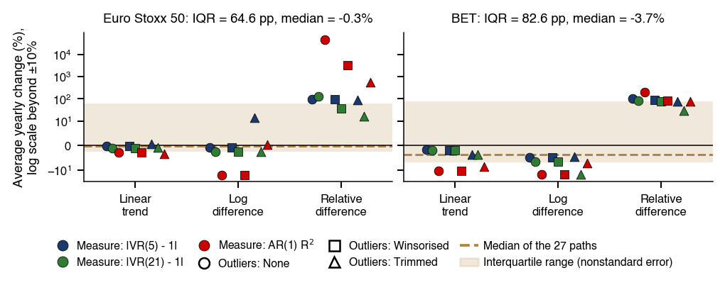
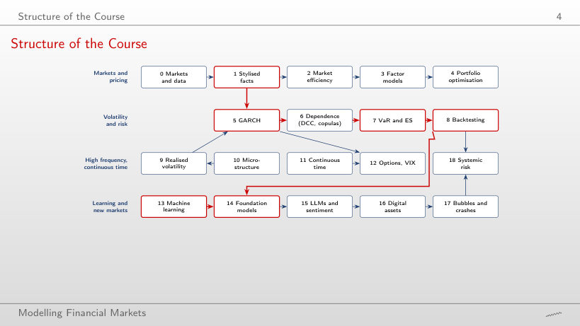
 MFM_ch19_case_study
 Statistics of Financial Markets